6  Ichthyop processes

In this section, the different Ichthyop processes are described. These processes are implemented in the classes within the action folder.

Parameters associated with these processes must be included in action blocks. They can be activated or deactivated by setting the enabled tag (cf. Section 3.1).

6.1 Activation/Deactivation of a process

Each process can be enabled or disabled by ticking on the enable tick box.

Furthermore, it is also possible to activate/deactivate some processes depending on the particle age (in days) or size (in \(cm\)).

This is done by providing, for each of these processes, the following parameters:

• activation_variable, which indicates whether age (in days) or length (in cm) must be used
• activation_minimum_class_value, which indicates the age (in days) or lengh (in cm) when the process becomes active. Default is 0
• activation_maximum_class_value, which indicates the age (in days) or lengh (in cm) when the process becomes inactive. Default is \(\infty\)

Caution

The length can be used only if one of the different growth process (see Section 6.3.2) is enabled

6.2 Transport processes

6.2.1 Advection

The primary process in Ichthyop is the advection by the ocean currents.

6.2.2 Horizontal advection

The particle grid coordinates will change according as follows:

\[ X(t + \Delta t) = X(t) + \frac{U \times \Delta t}{\Delta X} \]

\[ Y(t + \Delta t) = Y(t) + \frac{U \times \Delta t}{\Delta Y} \]

with \(X,Y\) the particle grid position, \(t\) the time, \(\Delta t\) the time step (in seconds), \(U\) and \(V\) the zonal and meridional velocities (in \(m.s^{-1}\)) and \(\Delta X\) and \(\Delta Y\) the zonal and meridional extent of the grid cell.

6.2.3 Vertical advection

For 3D simulations, vertical advection can also be activated. Particle depth, in grid coordinates, is given by:

\[ Z(t + \Delta t) = Z(t) + \frac{W \times \Delta t}{\Delta Z} \]

with \(Z\) the particle vertical grid position, \(t\) the time, \(\Delta t\) the time step (in seconds), \(W\) the vertical velocity (in \(m.s^{-1}\)) and \(\Delta Z\) the height of the grid cell.

6.2.4 Buoyancy

A buoyancy module allows to displace a particle vertically, depending on it’s density and the sea water density, following Parada et al. (2003).

The buoyancy-induced vertical velocity of the particle is given by:

\[ W_{buoy} = \dfrac{1}{24} \times g \times a \times b \times \dfrac{\rho_{water} - \rho_{part}}{\rho_{water}} \mu^{-1} \log\left(2 \dfrac{a}{b} + 0.5\right); \]

with \(a\) and \(b\) the semi-major axis and semi-minor axis of an ellipse (mean_major_axis and mean_minor_axis parameters), \(\mu\) the molecular viscosity (molecular_viscosity parameter), \(\rho_{water}\) the water density, \(\rho_{part}\) the particle density and \(g\) the gravitational acceleration (\(cm.s^{-2}\)).

There are two possibilities to define the particle buoyancy, which are provided by the density.method parameter:

• If constant, then a constant density (in \(g.cm^{-3}\)) is used, which is provided by the particle_density parameter.
• If file, then the buoyancy is read from a file and can vary with either age or length. The class that is used is provided by the density.class parameter.

The density CSV file must be formatted in the following way:

Age(Days);Density (g/cm3)
0;1.0235625
1;1.02374
2;1.023335
2.5;1.0239
2.75;1.025672

6.2.5 Daily vertical migration

Daily migration of the particles can be activated by providing daytime and nighttime depths, and the timing of the sunset and sunrise.

If the daytime_depth_file parameter is defined, it provides the depth of the particle during daytime. It is formatted as follows:

Age (day);Depth (m)
0.0;-20
3.0;-25
5.0;-30
8.0;-35

If this parameter is not found, a constant daytime depth, provided by the daytime_depth parameter, is assumed.

Same thing for the nighttime depths, which can be set by either the nighttime_depth_file or the nighttime_depth parameters.

The sunset and sunrise hours are set by the sunset and sunrise parameters, which must have a HH::mm format.

Warning

When the target depth is greater than the total depth, the particle does not move.

6.2.6 Horizontal dispersion

Horizontal dispersion is implemented following Peliz et al. (2007). The horizontal velocity component due to diffusion is:

\[ u_T = \delta \sqrt{\dfrac{2 K_h}{\Delta t}} \]

with \(\Delta t\) the time step, \(\delta\) a random number between -1 and 1 and \(K_h\) the imposed explicit Lagrangian horizontal diffusion.

The value of \(K_h\) depends on the mean mesh size where the particle is located:

\[ K_h = \epsilon^{1/3} l^{4/3} \]

with \(l\) is the mean mesh size and \(\epsilon\) is the turbulent dissipation rate (in \(m^2.s^{-3}\)).

In the Ichythop implementation (HDispAction.java), the displacement is computed:

\[ \Delta X = u_T \times \Delta t \]

Combining all together, we obtain the following equation:

\[ \Delta X = \delta \times \sqrt{\dfrac{2 \epsilon^{1/3} l^{4/3}}{\Delta t}} \times \Delta t \]

By putting the rightmost \(\Delta t\) within the square root, and by putting the \(l\) and \(\epsilon\) terms outside, this expression can be simplified as follows:

\[ \Delta X = \delta \times \sqrt{2 {\Delta t}} \times \epsilon^{1/6} \times l^{2/3} \]

The value of \(l\) is computing by averaging the mesh size along the \(X\) and \(Y\) dimensions.

6.2.7 Ontogenetic vertical migration

The ontogenetic migration module controls the migration of particles at different depths as a function of age. Its implementation in Ichthyop follows the CMS one. It uses a CMS configuration file, which is formatted as follows:

nTime
nDepth
z1 z2 z3 z4 z5 z6 ... znDepth
t1 t2 t3 t4 t5 t6 ... tnTime

P1,1 P1,2 ... P1,nTime
P2,1 P2,2 ... P2,nTime
P3,1 P3,2 ... P3,nTime
          ...
PnDepth,1 PnDepth,2 ... PnDepth,nTime

The first line provides the number of time steps in the CMS file, the second line provides the number of vertical levels in the CMS file. The third line provides the depth values and the fourth lines provides the time step values.

The remaining lines provide the probability matrix \(P_{z, t}\).

Note

The sum of the probability matrix along the depth dimension should equal 100.

At each time step, the index of the CMS time step, \(k\), is determined by comparing the simulation and CMS times as follows:

\[ t_{CMS}(k) < t \leq t_{CMS}(k + 1) \]

When the CMS time index changes, all the particles are randomly distributed on the vertical, following the probability distribution of the given CMS time. If the CMS time index remains unchanged, nothing is done.

6.2.8 Wind drift

The wind-drift is implemented in the WindDriftFileAction.java class. This class requires that 2D (time, latitude, longitude) wind fields are provided. This is done by providing a input_path and a file_filter parameters, which specify the location and names of the wind files.

The user also provides field_time, wind_u, wind_v, longitude, latitude parameters, which specify the names of the time, zonal wind, meridional wind, longitude and latitude variables in the NetCDF wind files.

The user also provides a depth_application parameter, which specifies the depth at which the wind will impact the trajectories (only valid for 3D simulations), a wind_factor (\(F\), multiplication factor), an angle (\(\theta\)) and a wind_convention parameter (\(\varepsilon\), +1 if convention is ocean-based, i.e. wind-to, -1 if convention is atmospheric based, i.e. wind-from).

The changes in particle longitude (\(\lambda\)) and latitude (\(\phi\)) is computed as follows:

\[ \Delta \lambda_0 = \frac{\Delta t \times U_W }{\frac{R \pi}{180} \times \cos(\frac{\pi \phi}{ 180})} \]

\[ \Delta \phi_0 = \frac{\Delta t \times V_W}{ \frac{R \pi}{180}} \]

\[ \Delta \lambda = \varepsilon \times F \times \left(\Delta \lambda_0 \times \cos\left(\frac{\theta \pi}{180}\right) - \Delta \phi_0 \times \sin\left(\frac{\theta \pi}{180}\right)\right) \]

\[ \Delta \phi = \varepsilon \times F \times \left(\Delta \lambda_0 \times \sin\left(\frac{\theta \pi}{180}\right) + \Delta \phi_0 \times \sin\left(\frac{\theta \pi}{180}\right)\right) \]

where \(\Delta \lambda_{0}\) and $_{0} $ are the changes in longitudes and latitudes due to wind, \(\Delta \lambda\) and $$ are the effective changes in longitudes and latitudes of the particle when taking into account the angle \(\theta\), \(\Delta t\) is Ichthyop time-step (in days) and \(U_w\) and \(V_w\) are the zonal and meridional wind components (in \(m.s^{-1}\)).

Note

\(R\) is the Earth Radius and equals 6367.74 km. In the code, \(\dfrac{R \pi}{180}\), which is the distance in m of a 1 degree cell, is approximated to 111138 m

6.2.9 Random swimming

Ichthyop allows particles to randomly swim. This is achieved by using the SwimmingAction.java. The velocity may vary with the age of the particle.

The user provides a CSV absolute velocity file (velocity_file parameter), which must me formatted as follows:

Age (days);Speed (m/s)
0;0.1
5;0.2
15;0.3

The user also provides a boolean parameter (constant_velocity) that specifies whether the velocity should remain as defined in the CSV file, or if the absolute velocity should be randomly selected as follows:

\[ \|U\| = \|U\|_{file} \times \kappa \]

with \(\kappa\) a random value in the \([0, 2]\) interval and \(\|U\|_{file}\) the velocity defined in the CSV file.

At each time-step, the zonal and meridonal velocities are defined as follows:

\[ U = \kappa' \varepsilon \|U\| \]

\[ V = \varepsilon' \sqrt{\|U\|^2 - U^2} \]

with \(\kappa'\) a random value between 0 and 1, and \(\varepsilon\) and \(\varepsilon'\) random values either equal to 1 or -1.

6.2.10 Wave drift

Ichthyop can take into account the effects of waves on the particles trajectories, following the Stokes drift equations (Stokes (2009)):

\[ U_{S} = w \times k_{wave} \times a^2 \times \exp\left(2 \times k_{wave} \times z\right) \]

where \(w \times k \times a^2\) is the Stokes drift velocity, \(k_{wave}\) is the wave number and \(z\) is the depth.

In Ichthyop, the user provides the zonal and meridional components of the Stokes drift (\(U_{stokes}\) and \(V_{stokes}\)), the zonal and meridional wave velocities (\(U_{wave}\) and \(V_{wave}\)) and the wave period (\(T_{wave}\)).

Important

Note that all the fields provided by the user are 2D!

First, the value of \(k_{wave}\) is computed from the wave velocity and the wave period:

\[ \|U_{wave}\| = U_{wave}^2 + V_{wave}^2 \]

\[ \lambda_{wave} = \|U_{wave}\| \times T_{wave} \]

\[ k_{wave} = \dfrac{2 \pi}{\lambda_{wave}} \]

Then, the horizontal displacement due to the Stokes drift is computed as follows:

\[ \Delta X = F \times U_{stokes} \times \Delta t \times \exp\left(2 \times k_{wave} \times z\right) \]

\[ \Delta Y = F \times V_{stokes} \times \Delta t \times \exp\left(2 \times k_{wave} \times z\right) \]

with \(k_{wave}\) the wave number as computed above, \(U_{stokes}\) and \(V_{stokes}\) the zonal and meridional components of the Stokes drift, \(z\) the depth and \(F\) a multiplication factor provided by the user.

6.2.11 Rafting

The rafting process allows a particle to move at the surface, given a certain age, in order to take benefic from the ocean currents.

In Ichthyop implementation, when a particle reaches a certain age or size, then the particle is moved at the surface and will remain there.

6.2.12 Coastal behaviour

Coastal behaviour defines what is done before aplying the change in location to an Ichthyop particle

6.2.12.1 Default

The default behavior is to do nothing prior the displacement of a particle. The change in coordinate of the particle is applied whatsoever, and the particle may be inland. It remains alive but then its behavior is uncertain.

Warning

It is strongly advised not to use this default mode

6.2.12.2 Beaching

Before the particle is moved, Ichthyop checks whether the coming displacement will bring the particle inland. If so, the particle is moved and then is killed, with the BEACHED mortality status.

6.2.12.3 Standstill

Before the particle is moved, Ichthyop checks whether the coming displacement will bring the particle inland. If so, its deplacement is cancelled and the particle remains at the same position until a new displacement brings it in a water cell.

6.2.12.4 Bouncing

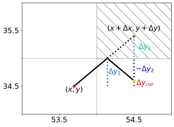
In the bouncing mode, Ichthyop will check whether the displacement will bring the particle inland. If so, the particle will bounce on the coast. First, whether the bouncing occurs on a meridional or a zonal coastline is determined.

In case of a meridional coastline, as shown in Figure 6.1, the calculation of the new position is performed as follows.

Let’s assume that the particle is at the position \((x, y)\) and would normally move at the postion \((x + \Delta x, y + \Delta y)\). We suppose that

\[ \Delta y = \Delta y_1 + \Delta y_2, \tag{6.1}\]

where \(\Delta y_1\) is the meridional distance between the particle and the coastline, and \(\Delta y_2\) is the distance that the particle would travel on land.

In the bouncing mode, the position increment can be written as

\[ \Delta y_{cor} = \Delta y_1 - \Delta y_2 \tag{6.2}\]

By replacing \(\Delta y_2\) using Equation 6.1, we can write:

\[ \Delta_{cor} y = \Delta y_1 - (\Delta y - \Delta y_1) \]

\[ \Delta_{cor} y = 2 \Delta y_1 - \Delta y \]

Figure 6.1: Coastal behaviour in bouncing mode.

6.3 Biological processes

6.3.1 Orientation

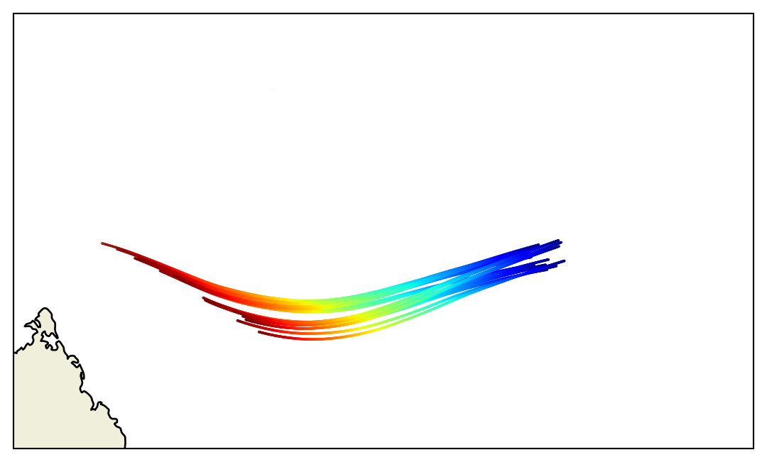
Active swimming has been implemented in Ichthyop following the work of Romain Chaput. Three active swimming behaviours have been implemented: the rheotaxis orientation (i.e. against the current), the cardinal orientation (i.e toward a given direction) and the reef orientation, i.e. orientation toward points of interests.

These three implementations involve the computation of a swimming velocity and direction. The former is common to all three methods, but the directions depend on the method considered.

import xarray as xr
import cartopy.crs as ccrs
import cartopy.feature as cfeature
import os
from glob import glob
import matplotlib.pyplot as plt
import numpy as np
import matplotlib as mpl

config = 'control'

if os.path.isdir('ichthyop_output'):
    pattern = os.path.join('ichthyop_output', config, '*nc')
else :
    pattern = os.path.join('..', '..', 'ichthyop_output', config, '*nc')
pattern

filelist = glob(pattern)
filelist

data = xr.open_mfdataset(filelist, decode_times=False)
data

# +
lon = data['lon'].values
lat = data['lat'].values
mort = data['mortality'].values

lon = np.ma.masked_where(mort > 0, lon)
lat = np.ma.masked_where(mort > 0, lat)
ntime, ndrifters = lon.shape

# +
time = np.arange(ntime)
drifters = np.arange(ndrifters)

d2d, t2d = np.meshgrid(drifters, time)

# +
plt.figure()

projin = ccrs.PlateCarree()
projout = ccrs.PlateCarree()

ax = plt.axes(projection = projout)
ax.scatter(lon[:, :], lat[:, :], c=t2d, marker='.', transform=projin, s=0.5, cmap=mpl.colormaps['jet'])
feat = ax.add_feature(cfeature.LAND)
feat = ax.add_feature(cfeature.COASTLINE)
ax.set_extent([49, 55.25, -13.13, -9.45], crs=projin)

Figure 6.2: Trajectory without orientation

6.3.1.1 Swimming velocity

The orientation processes all share common features. They both depend on a swimming velocity and random directions. The methods described below differ on the way the random directions are drafted.

Swimming velocity is computed following Staaterman et al. (2012):

\[ V = V_{hatch} + (V_{settle} - V_{hatch}) ^ {\log(age) / \log(PLD)} \]

with \(V_{hatch}\) and \(V_{settle}\) the larval velocity at hatching and settle, \(A\) the age of the larva and \(PLD\) the transport duraction.

import matplotlib.pyplot as plt
import numpy as np
from scipy.special import i0

PLD = 10
x = np.linspace(0, PLD, 1000)[1:]

vhatch = 10
vsettle = 200

vel = vhatch + np.power(vsettle - vhatch, np.log10(x)/np.log10(PLD))

plt.figure()
plt.plot(x, vel)
plt.xlabel('Age (days)')
plt.ylabel('$V (cm.s^{-1})$')
plt.xlim(x.min(), x.max())
plt.title('$PLD = %dd, V_{hatch}=%d cm.s^{-1}, V_{settle}=%d cm.s^{-1}$' %(PLD, vhatch, vsettle))
plt.show()

6.3.1.2 Von Mises distributions

Von Mises distribution is used in all three methods.The Von Mises distribution is given by:

\[ f(\theta, \mu, \kappa) = \dfrac {\exp(\kappa \cos(\theta - \mu))} {2 \pi I_{0}(\kappa)} \]

where \(I_{0}(\kappa)\) is the modified Bessel function of the first kind of order 0, \(\mu\) is angle where the distribution is centerred and \(\kappa\) is the concentration parameter. The distribution is as follows:

import matplotlib.pyplot as plt
import numpy as np
from scipy.special import i0

x = np.linspace(-np.pi, np.pi, 200)

def von_misses(kappa):
    mu = 0
    y = np.exp(kappa*np.cos(x-mu))/(2*np.pi*i0(kappa))
    return y

plt.figure()

for i in [0.5, 1, 2, 5, 10, 20]:
    plt.plot(x, von_misses(i), label=f'$\kappa = {i}$')
plt.legend()
plt.xlim(x.min(), x.max())
plt.show()

<>:15: SyntaxWarning: invalid escape sequence '\k'
<>:15: SyntaxWarning: invalid escape sequence '\k'
/tmp/ipykernel_4097/2623890059.py:15: SyntaxWarning: invalid escape sequence '\k'
  plt.plot(x, von_misses(i), label=f'$\kappa = {i}$')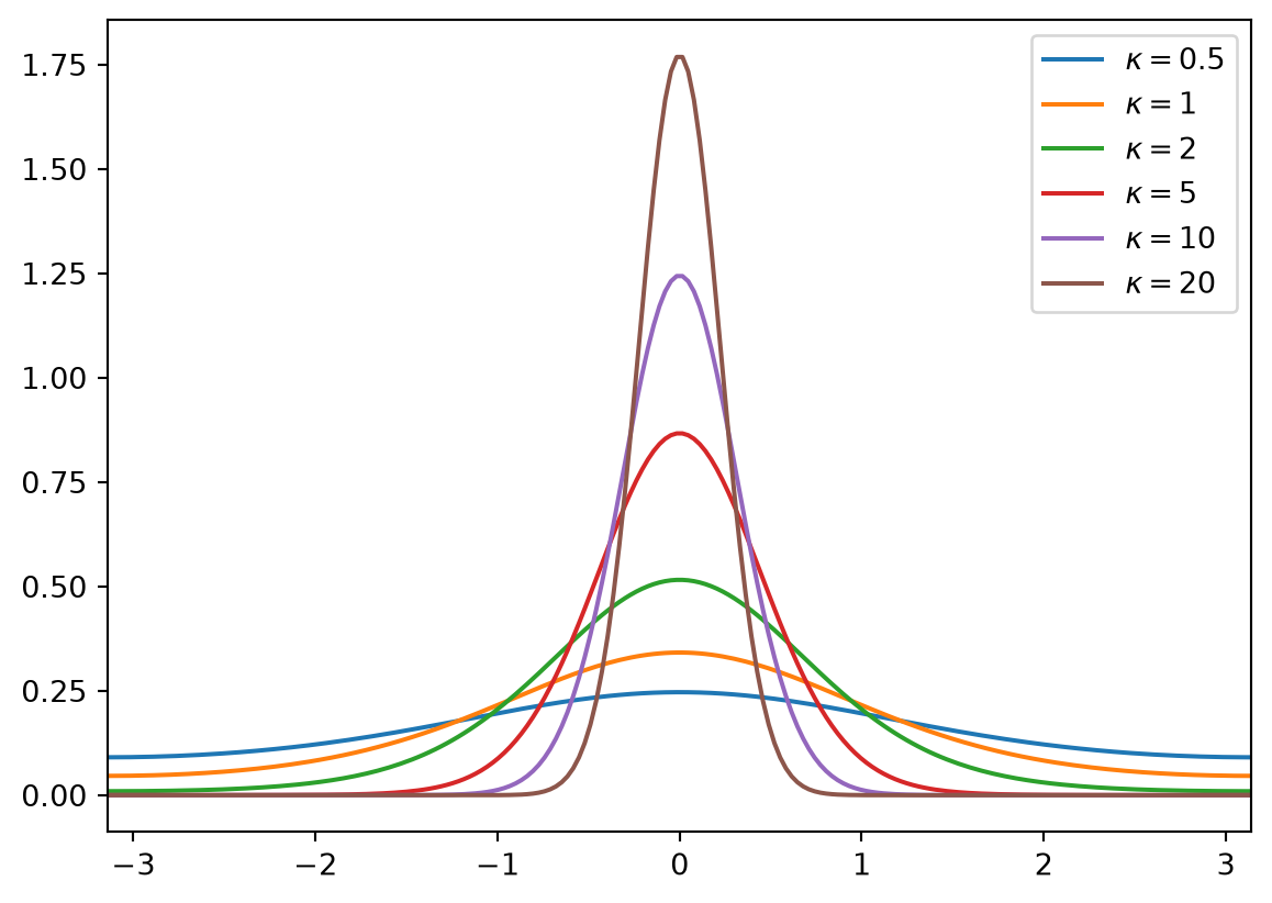

For computation purposes, all the Von Mises drafts performed in Ichthyop are done by using \(mu = 0\). The angles are thus centerred around 0. Then, the \(mu\) value is added.

Note

\(\theta = 0\) is eastward, \(\theta = \frac{\pi}{2}\) is northward, etc.

6.3.1.3 Computation of displacement

Given a swimming velocity \(V\) and a direction \(\theta\), the larva displacement (in \(m\)) is computed as follows:

\[ \Delta X = V \times \cos(\theta) \times \Delta t \]

\[ \Delta Y = V \times \sin(\theta) \times \Delta t \]

with \(\Delta t\) the time step. Next, the corresponding change in longitude (\(\lambda\)) and latitude (\(\varphi\)) is computed as follows:

\[ \Delta \lambda = \dfrac{\Delta X}{111138 \times \cos{\varphi}} \]

\[ \Delta \varphi = \dfrac{\Delta Y}{111138 } \]

6.3.1.4 Cardinal orientation

In cardinal orientation, the user provides a fixed heading \(\theta_{card}\) and a fixed \(\kappa\) parameter. Then, at each time step, a new angle is randomly drafted following a Von Misses distribution \(f(\theta, \theta_{card}, \kappa)\).

import xarray as xr
import cartopy.crs as ccrs
import cartopy.feature as cfeature
import os
from glob import glob
import matplotlib.pyplot as plt
import numpy as np
import matplotlib as mpl

config = 'card'

if os.path.isdir('ichthyop_output'):
    pattern = os.path.join('ichthyop_output', config, '*nc')
else :
    pattern = os.path.join('..', '..', 'ichthyop_output', config, '*nc')
pattern

filelist = glob(pattern)
filelist

data = xr.open_mfdataset(filelist, decode_times=False)
data

# +
lon = data['lon'].values
lat = data['lat'].values
mort = data['mortality'].values

lon = np.ma.masked_where(mort > 0, lon)
lat = np.ma.masked_where(mort > 0, lat)
ntime, ndrifters = lon.shape

# +
time = np.arange(ntime)
drifters = np.arange(ndrifters)

d2d, t2d = np.meshgrid(drifters, time)

# +
plt.figure()

projin = ccrs.PlateCarree()
projout = ccrs.PlateCarree()

ax = plt.axes(projection = projout)
ax.scatter(lon[:, :], lat[:, :], c=t2d, marker='.', transform=projin, s=0.5, cmap=mpl.colormaps['jet'])
feat = ax.add_feature(cfeature.LAND)
feat = ax.add_feature(cfeature.COASTLINE)
ax.set_extent([49, 55.25, -13.13, -9.45], crs=projin)

6.3.1.5 Rheotaxis orientation

In the rheotaxis orientation method, the particles swim against the current. The user only provides a kappa parameter.

First, the angle of the current is computed as follows:

\[ \theta_{current} = \arctan2(V_{current}, U_{current}) \]

Then, the angle that the particle must follow is given by adding \(\pi\):

\[ \theta_{direction} = \theta_{current} + \pi \]

Finally, a random angle is picked up following a Von Mises distribution \(f(\theta, \theta_{direction}, \kappa_{reef})\)

(ref-rheo)=

import xarray as xr
import cartopy.crs as ccrs
import cartopy.feature as cfeature
import os
from glob import glob
import matplotlib.pyplot as plt
import numpy as np
import matplotlib as mpl

config = 'rheo'

if os.path.isdir('ichthyop_output'):
    pattern = os.path.join('ichthyop_output', config, '*nc')
else :
    pattern = os.path.join('..', '..', 'ichthyop_output', config, '*nc')
pattern

filelist = glob(pattern)
filelist

data = xr.open_mfdataset(filelist, decode_times=False)
data

# +
lon = data['lon'].values
lat = data['lat'].values
mort = data['mortality'].values

lon = np.ma.masked_where(mort > 0, lon)
lat = np.ma.masked_where(mort > 0, lat)
ntime, ndrifters = lon.shape

# +
time = np.arange(ntime)
drifters = np.arange(ndrifters)

d2d, t2d = np.meshgrid(drifters, time)

# +
plt.figure()

projin = ccrs.PlateCarree()
projout = ccrs.PlateCarree()

ax = plt.axes(projection = projout)
ax.scatter(lon[:, :], lat[:, :], c=t2d, marker='.', transform=projin, s=0.5, cmap=mpl.colormaps['jet'])
feat = ax.add_feature(cfeature.LAND)
feat = ax.add_feature(cfeature.COASTLINE)
ax.set_extent([49, 55.25, -13.13, -9.45], crs=projin)

6.3.1.6 Reef orientation

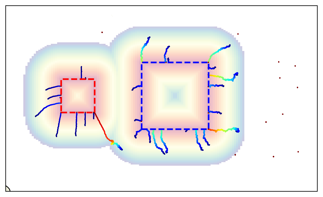
In the reef orientation method, the larva will target the closest target area (for instance coral reef). These areas are defined in an XML zone file by a polygon and a zone-specific \(\kappa\) parameter. The user also provides the sensory detection threshold of the larva (maximum detection distance \(\beta\)).

If the distance between the particle and the barycenter of the closest reef (\(D\)) is below the detection thereshold \(\beta\), the larva will swim in the direction of the reef.

(ref-orientation)=

import numpy as np
import matplotlib.pyplot as plt

plt.rcParams['font.size'] = 15

plt.figure(figsize = (10, 10))

xnew = 0
ynew = 0

#draw point at orgin
plt.plot(xnew, ynew, color = 'red', marker = 'o')
plt.gca().annotate('$P_{t}$', xy=(0 + 0.05, 0 - 0.07), xycoords='data', color='red')

#draw circle
r = 1.5
angles = np.linspace(0 * np.pi, 2 * np.pi, 100 )
xs = r * np.cos(angles)
ys = r * np.sin(angles)
plt.plot(xs, ys, color = 'k', ls='--', lw=0.5)

angle_old = np.pi / 6.
rold = 1.
xold = rold * np.cos(angle_old)
yold = rold * np.sin(angle_old)

plt.plot(xold, yold, marker='o', color='blue')
plt.gca().annotate('$P_{t - 1}$', xy=(xold + 0.05, yold), xycoords='data', color='blue')

angle_reef = np.pi + np.pi / 3.
print(np.rad2deg(angle_reef))
rreef = 1
xreef = rreef * np.cos(angle_reef)
yreef = rreef * np.sin(angle_reef)
print(yreef)

plt.plot(xreef, yreef, marker='o', color='orange')
plt.gca().annotate('$R$', xy=(xreef + 0.1, yreef), xycoords='data', color='orange')

plt.gca().annotate(r'$D$', xy=(0.5*(xreef) + 0.02, 0.5*yreef), xycoords='data', color='orange', ha='left')

plt.axvline(xnew, color='k', ls='--', lw=0.5)
plt.axhline(ynew, color='k', ls='--', lw=0.5)

p = np.polyfit([xold, xnew], [yold, ynew], deg=1)
xtemp = np.linspace(xold, xold -2, 100)
plt.plot(xtemp, np.polyval(p, xtemp), color='black', ls='--')

angle_current = angle_old + np.pi
tmp_angle = np.linspace(0, angle_current, 100)
rtmp = 0.2
plt.plot(0 + rtmp * np.cos(tmp_angle), 0 + rtmp * np.sin(tmp_angle), color='k', ls='--')
plt.gca().annotate(r'$\theta_{actual}$', xy=(xnew + 0.2, ynew+0.05), xycoords='data', color='k')


plt.plot([xnew, xreef], [ynew, yreef], color='orange', ls='--')
angle_current = angle_reef
tmp_angle = np.linspace(0, angle_current, 100)
rtmp = 0.3
plt.plot(0 + rtmp * np.cos(tmp_angle), 0 + rtmp * np.sin(tmp_angle), color='orange', ls='--')
plt.gca().annotate(r'$\theta_{reef}$', xy=(xnew - 0.3, ynew+0.1), xycoords='data', color='orange',ha='right')

angle_current = angle_old + np.pi
tmp_angle = np.linspace(angle_current, angle_reef, 100)
rtmp = 0.4
plt.plot(0 + rtmp * np.cos(tmp_angle), 0 + rtmp * np.sin(tmp_angle), color='plum', ls='--')
plt.gca().annotate(r'$\theta_{turning}$', xy=(-0.43, -0.34), xycoords='data', color='plum')

off = 0.05
plt.xlim(xreef - off, xold + off)
plt.ylim(yreef - off, yold + off)
plt.gca().set_aspect('equal')
plt.axis('off')
plt.show()

239.99999999999997
-0.8660254037844384

First, the angle of the current trajectory, \(\theta_{actual}\), is computed by using the particle position at the previous time step (blue point) and the actual position (red point).

\[ \Delta_X = (X_{t - 1} - X_{t}) \]

\[ \Delta_Y = (Y_{t - 1} - Y_{t}) \]

\[ \theta_{actual} = \arctan2(\Delta Y, \Delta X) + \pi \]

The direction toward the reef, \(\theta_{reef}\) is also computed.

\[ \Delta_X = (X_{reef} - X_{t}) \]

\[ \Delta_Y = (Y_{reef} - Y_{t}) \]

\[ \theta_{reef} = \arctan2(\Delta Y, \Delta X) \]

Warning

The angles are computed in the \((X, Y)\) space. Therefore, longitude and latitude coordinates are converted in \((X, Y)\) using the latlon2xy Dataset methods.

The turning angle \(\theta_{turning}\) is given by:

\[ \theta_{turning} = \theta_{reef} - \theta_{actual} \]

The turning angle is then ponderated by the ratio of the distance from the reef to the detection threshold as follows:

\[ \theta_{ponderated} = \left(1 - \dfrac{D}{\beta}\right) \theta_{turning} \]

\[ \theta_{ponderated} = \left(1 - \dfrac{D}{\beta}\right) \left(\theta_{reef} - \theta_{actual}\right) \]

Therefore, the closest to the reef, the strongest the turning angle.

Then, a random angle is picked up following a Von Mises distribution \(f(\theta, \theta_{ponderated}, \kappa_{reef})\)

An example of a trajectory is provided below. In this case, two target destinations are provided (black boxes). The same \(\kappa\) value was used for both ares (1.2) and the \(\beta\) parameter has been set equal to 3 km.

(ref-orientation-2)=

import xarray as xr
import cartopy.crs as ccrs
import cartopy.feature as cfeature
import os
from glob import glob
import matplotlib.pyplot as plt
import numpy as np
import matplotlib as mpl

config = 'reef'

if os.path.isdir('ichthyop_output'):
    pattern = os.path.join('ichthyop_output', config, '*nc')
else :
    pattern = os.path.join('..', '..', 'ichthyop_output', config, '*nc')
pattern

filelist = glob(pattern)
filelist

data = xr.open_mfdataset(filelist, decode_times=False)
data

# +
lon = data['lon'].values
lat = data['lat'].values
mort = data['mortality'].values

lon = np.ma.masked_where(mort > 0, lon)
lat = np.ma.masked_where(mort > 0, lat)
ntime, ndrifters = lon.shape

# +
time = np.arange(ntime)
drifters = np.arange(ndrifters)

d2d, t2d = np.meshgrid(drifters, time)

# +
plt.figure()

projin = ccrs.PlateCarree()
projout = ccrs.PlateCarree()

ax = plt.axes(projection = projout)
ax.scatter(lon[:, :], lat[:, :], c=t2d, marker='.', transform=projin, s=0.5, cmap=mpl.colormaps['jet'])
feat = ax.add_feature(cfeature.LAND)
feat = ax.add_feature(cfeature.COASTLINE)
xp = np.array([51.625, 52.625, 52.625,51.625, 51.625])
yp = np.array([-1.179878E1, -1.179878E1, -1.079878E1, -1.079878E1, -1.179878E1])
ax.plot(xp, yp, transform=projin, color='k', ls='--')
xp = np.array([51.625, 52.625 - 0.5, 52.625 - 0.5,51.625, 51.625]) - 1
yp = np.array([-1.179878E1 + 0.5, -1.179878E1 + 0.5, -1.079878E1, -1.079878E1, -1.179878E1 + 0.5]) - 0.25
ax.plot(xp, yp, transform=projin, color='k', ls='--')
ax.set_extent([49, 55.25, -13.13, -9.45], crs=projin)

6.3.2 Growth

There are 3 different implementations of the growth module. They can be selected by setting the class_name parameter in the action.growth action configuration block.

6.3.2.1 Linear growth

In the linear growth method described in Lett et al. (2008), length depends on temperature but may also depend on the available food if the growth.food.enabled parameter is set to True.

If food dependence is enabled, length increment (in \(cm\)) is given by:

\[ \Delta L = C1 + C2 \times \dfrac{F}{F + K_S} \times max(T, T_{thres}) \times \Delta t \]

where \(\Delta t\) is the time-step (in seconds), \(C1\) and \(C2\) are parameters (coeff1 and coeff2), \(T_{thres}\) is a temperature threshold (threshold_temp parameter), \(F\) is the food quantity (read from a biogeochemical dataset), and \(K_S\) is a half-saturation constant (half_saturation parameter) and \(T\) is the temperature (read from the hydrodynamic dataset).

If food dependence is disabled, then increment is provided as follows:

\[ \Delta L = C1 + C2 \times max(T, T_{thres}) \times \Delta t \]

The name of the food and temperature variables are provided by the food_field and temperature_field parameters.

The initial length of the particle is provided by the initial_length parameter.

6.3.2.2 Sole growth

In the Sole growth model used in Tanner et al. (2017), length increment (in \(cm\)) relies on the growth equation from Fonds (1979) :

\[ \Delta L = C1 \times T^{C2} \times \Delta t \]

with \(L\) the length (in \(cm\)), \(T\) the temperature and \(\Delta t\) the time step seconds, and \(C1\) and \(C2\) are parameters (c1 and c2 respectively).

The temperature field is provided by the temperature_field parameter.

6.3.2.3 Exponential growth

In the exponential model, length is given by the following equation:

\[ L(t) = L_0 \times \exp{\left(b T^c t\right)} \]

with \(L_0\) the initial length (in cm), \(b\) the growth rate and \(c\) the temperature dependence of the growth rate.

Taking the derivative of this expression, we obtain the length increment (in \(cm\)) as a function of time:

\[ \Delta L = L \times b \times T^{c} \times \Delta t \]

The initial length of the particle is provided by the initial_length parameter.

6.3.3 Lethal temperature and salinity

In Ichthyop, there is the possibility to define temperature and salinity values below and above which the particle is killed.

The same set of parameters are used in both cases, with the temperature and salinity prefix. There are two ways to define lethal temperatures and salinities:

• Using constant lethal temperatures or salinities (if temperature.file.enabled or salinity.file.enabled is set to false)
• Using a CSV file containing lethal temperatures or salinities as a function of the particle class.

If constant lethal temperatures or salinities are provided, the cold and warm lethal temperatures are provided with the cold_lethal_temperature, warm_lethal_temperature, fresh_lethal_salinity, saline_lethal_salinity, .

If a CSV file is used, the lethal temperatures and salinities are provided in a CSV (lethal_temperature_file and lethal_salinity_file parameters) which is formatted as follows:

Age(days);Cold temperature (C);Warm temperature (C)
0;14;22
2;13;22
6;12;22

The first column provides the class intervals, which are either the age of the particle (in days) or the length of the particle (in cm). The variable that is used to determine the class is provided by the temperature.class parameter.

6.3.3.1 DEB growth

The DEB equations are based on Kooijman (2010) and can be found in Flores-Valiente et al. (2023)

Influence of temperature is given by equation 5 of Flores-Valiente et al. (2023):

\[ c_T = \exp \left( \dfrac{T_A}{T_1} - \dfrac{T_A}{T} \right) \left[ \dfrac{ 1 + \exp \left( \dfrac{T_{AL}}{T_1} - \dfrac{T_{AL}}{T_L} \right) + \exp \left( \dfrac{T_{AH}}{T_H} - \dfrac{T_{AH}}{T_1} \right) } { 1 + \exp \left( \dfrac{T_{AL}}{T} - \dfrac{T_{AL}}{T_L} \right) + \exp \left( \dfrac{T_{AH}}{T_H} - \dfrac{T_{AH}}{T} \right) } \right] \tag{6.3}\]

If the particle is an embryo (\(E_H < E_{Hb}\)), then it does not feed. Please note that, according to this definition, a larva that hatched but does not feed is considered an embryo in DEB theory. Else, the scaled functional response \(f\) is computed as:

\[ f = \dfrac{F}{F + K} \tag{6.4}\]

with \(F\) the food vector and \(K\) the half-saturation constant.

Assimilation rates \(\{\dot{p_{Am}}\}\), energy conductance \(\dot{v}\), volume specific somatic maintenance (\([\dot{p}_M]\)) and maturity maintenances rates (\(\dot{k}_J\)) are corrected by the \(c_T\) factor.

If the accelerated DEB model is used (see e.g. Kooijman et al. (2011) and Kooijman (2014) for more details), the acceleration factor is computed as follows

\[ s_M = \begin{cases} 1 & (E < E_{Hb})\\ \dfrac{V^{1/3}}{L_b} & (E_{Hb} \le E_H < E_{Hj}) \\ \dfrac{L_j}{L_b} & (E_{H} > E_{Hj}) \end{cases} \tag{6.5}\]

with \(L_b\) the structural length of the particle when \(E_H = E_Hb\) (i.e the length at birth, i.e. first feeding) and \(L_j\) the structural length of the particle when \(E_H = E_Hj\) (i.e the length when metamorphosis occurs). The \(s_M\) factor is then used to multiply the assimilation rate \(\{\dot{p_{Am}}\}\) and the energy conductance \(\dot{v}\).

(NICOLAS: s’agit il de la longueur structurelle \(L = V^{1/3}\) ou de la longueur mesurée \(L_w = L / \delta_M\)). Please note that \(L_b\) and \(L_j\) are here considered as parameters but they should be in fact calculated prior any Ichthyop runs at (e.g. at \(f = 1\)) as they depend on the other parameters. If you are considering testing different parameter sets, \(L_b\) and \(L_j\) should be modified accordingly (e.g. using the DEBtool function get_tj.m).

Consequently, the assimilation (in \(J.d^{-1}\)) is computed as follows:

\[ \dot{p}_A = \begin{cases} 0 & (E_{H} < E_{Hb}) \\ c_T s_M f \{ \dot{p}_{Am}\} V^{2/3} & (E_{H} \ge E_{Hb}) \\ \end{cases} \tag{6.6}\]

Energy loss to maintenance is given by

\[ \dot{p}_M = c_T [ \dot{p}_M ] V \tag{6.7}\]

The mobilized energy is given by:

\[ \dot{p_C} = c_T \dfrac{\dfrac{E}{V} \left([E_G] s_M \dot{v} V^{2/3} + \dot{p}_M\right)} {\kappa \dfrac{E}{V} + [E_G]} \tag{6.8}\]

Maturity maintenance is given by

\[ \dot{p}_J = c_T \dot{k}_J E_H \tag{6.9}\]

Energy that is sent to structural growth is given by:

\[ \dot{p}_G = \kappa \dot{p}_C - \dot{p}_M \tag{6.10}\]

Energy that goes to development (as embryo and juvenile) or to reproduction (as adults) is given by:

\[ \dot{p}_R = (1 - \kappa) \dot{p}_C - \dot{p}_J \tag{6.11}\]

Finally, the increment of reserve \(E\) and structural volume \(V\) is given by:

\[ \dfrac{dE}{dt} = \dot{p}_A - \dot{p}_C \tag{6.12}\]

\[ \dfrac{dV}{dt} = \dfrac{\dot{p}_G}{{[E_G]}} \tag{6.13}\]

The increment of the energy invested into development or reproduction depends on the value of \(E_H\).

\[ \dfrac{dE_H}{dt} = \begin{cases} \dot{p}_R & E_H < E_{Hp}\\ 0 & \text{otherwise} \end{cases} \tag{6.14}\]

\[ \dfrac{dE_R}{dt} = \begin{cases} 0 & E_H < E_{Hp}\\ \dot{p}_R & \text{otherwise} \end{cases} \tag{6.15}\]

Finally, starvation mortality is determined whether one of the following conditions are matched:

\[ M_{starv} = \begin{cases} \kappa \dot{p}_C < \dot{p}_M\\ (1 - \kappa) \dot{p}_C < \dot{p}_J \end{cases} \tag{6.16}\]

Finally, all the states variables are then incremented:

\[ E(t + \Delta t) = E(t) + \dfrac{dE}{dt}\Delta t \tag{6.17}\]

\[ V(t + \Delta t) = V(t) + \dfrac{dV}{dt}\Delta t \tag{6.18}\]

\[ E_H(t + \Delta t) = E_H(t) + \dfrac{dE_H}{dt}\Delta t \tag{6.19}\]

\[ E_R(t + \Delta t) = E_R(t) + \dfrac{dE_R}{dt}\Delta t \tag{6.20}\]

Additional references

Kooijman, S. A. L. M. (2010). Dynamic Energy Budget theory for metabolic organisation. Cambridge Univ. Press, Cambridge. doi: 10.1098/rstb.2010. Kooijman, S. A. L. M. (2014). Metabolic acceleration in animal ontogeny: An evolutionary perspective. Journal of Sea Research, 94(Supplement C), 128–137. https://doi.org/10.1016/j.seares.2014.06.005 Kooijman, S. A. L. M., Pecquerie, L., Augustine, S., & Jusup, M. (2011). Scenarios for acceleration in fish development and the role of metamorphosis. J. Sea Res., 66, 419–423. https://doi.org/10.1016/j.seares.2011.04.016

(book?){kooijman_dynamic_2010, title = {Dynamic {Energy} {Budget} theory for metabolic organisation}, isbn = {978-0-521-13191-9}, url = {doi: 10.1098/rstb.2010.}, publisher = {Cambridge Univ. Press, Cambridge}, author = {Kooijman, S.A.L.M.}, year = {2010}, }

(article?){kooijman_scenarios_2011, title = {Scenarios for acceleration in fish development and the role of metamorphosis.}, volume = {66}, doi = {https://doi.org/10.1016/j.seares.2011.04.016}, journal = {J. Sea Res.}, author = {Kooijman, S. A. L. M. and Pecquerie, L. and Augustine, S. and Jusup, M.}, year = {2011}, pages = {419–423}, }

(article?){kooijman_metabolic_2014, series = {Dynamic {Energy} {Budget} theory: applications in marine sciences and fishery biology}, title = {Metabolic acceleration in animal ontogeny: {An} evolutionary perspective}, volume = {94}, issn = {1385-1101}, shorttitle = {Metabolic acceleration in animal ontogeny}, url = {http://www.sciencedirect.com/science/article/pii/S1385110114001105}, doi = {10.1016/j.seares.2014.06.005}, number = {Supplement C}, urldate = {2017-11-21}, journal = {Journal of Sea Research}, author = {Kooijman, S. A. L. M.}, month = nov, year = {2014}, keywords = {Acceleration, Dispersal, Maturation, Parental care, add_my_pet}, pages = {128–137}, }

Flores-Valiente, Jorge, Christophe Lett, François Colas, et al. 2023. “Influence of Combined Temperature and Food Availability on Peruvian Anchovy (Engraulis Ringens) Early Life Stages in the Northern Humboldt Current System: A Modelling Approach.” Progress in Oceanography 215: 103034. https://doi.org/https://doi.org/10.1016/j.pocean.2023.103034.

Fonds, M. 1979. “Laboratory Observations on the Influence of Temperature and Salinity on Development of the Eggs and Growth of the Larvae of Solea Solea (Pisces).” Mar. Ecol. Prog. Ser 1 (9).

Lett, Christophe, Philippe Verley, Christian Mullon, et al. 2008. “A Lagrangian Tool for Modelling Ichthyoplankton Dynamics.” Environmental Modelling & Software 23 (9): 1210–14. https://doi.org/https://doi.org/10.1016/j.envsoft.2008.02.005.

Parada, C, CD Van Der Lingen, C Mullon, and P Penven. 2003. “Modelling the Effect of Buoyancy on the Transport of Anchovy (Engraulis Capensis) Eggs from Spawning to Nursery Grounds in the Southern Benguela: An IBM Approach.” Fisheries Oceanography 12 (3): 170–84.

Peliz, Alvaro, Patrick Marchesiello, Jesus Dubert, Martinho Marta-Almeida, Claude Roy, and Henrique Queiroga. 2007. “A Study of Crab Larvae Dispersal on the Western Iberian Shelf: Physical Processes.” Journal of Marine Systems 68 (1): 215–36. https://doi.org/https://doi.org/10.1016/j.jmarsys.2006.11.007.

Staaterman, Erica, Claire B. Paris, and Judith Helgers. 2012. “Orientation Behavior in Fish Larvae: A Missing Piece to Hjort’s Critical Period Hypothesis.” Journal of Theoretical Biology 304 (July): 188–96. https://doi.org/10.1016/j.jtbi.2012.03.016.

Stokes, George Gabriel. 2009. “On the Theory of Oscillatory Waves.” In Mathematical and Physical Papers, vol. 1. Cambridge Library Collection - Mathematics. Cambridge University Press. https://doi.org/10.1017/CBO9780511702242.013.

Tanner, Susanne E., Ana Teles-Machado, Filipe Martinho, Álvaro Peliz, and Henrique N. Cabral. 2017. “Modelling Larval Dispersal Dynamics of Common Sole (Solea Solea) Along the Western Iberian Coast.” Progress in Oceanography 156: 78–90. https://doi.org/https://doi.org/10.1016/j.pocean.2017.06.005.