2 Ichthyop user interface (beginners)
When Ichthyop is ran with its user interface, a simulation comprises 4 steps
- configuration (Section 2.1)
- running (Section 2.2)
- visualize results (Section 2.3)
- and animation (Section 2.4).
2.1 Configuration
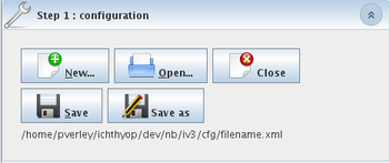
Firstly you will find the usual “File menu” functions : create a new configuration file, open an existing one, close it and save it.
2.1.1 New configuration file
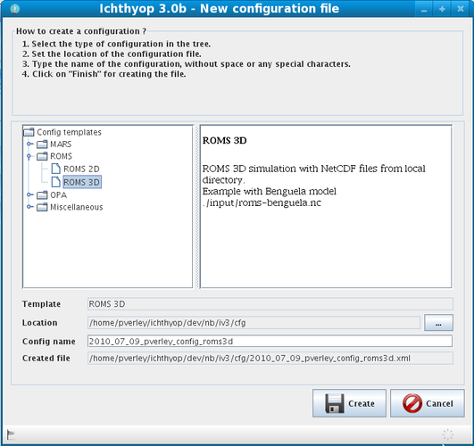
The application comes with some preset examples of configuration files (i.e. the templates). Select one of the templates, change the name of the configuration if the suggested name does not suit you and click on the Create button.
2.1.2 Content of the configuration file
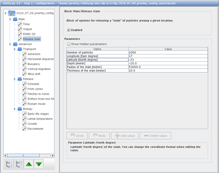
The configuration file is organized in several categories and each category contains several blocks of parameters.
Main blocks:
- Time: Set the simulation time options, such as the beginning of the simulation, the duration of transport, the time step, etc.
- Output: Options that control the record of the particle tracks in a NetCDF output file.
- Dataset (e.g. ROMS 3D): Management of the hydrodynamic dataset (which comes as inputs of Ichthyop).
- Release: Determine how and where the particles should be released (see Chapter 5)
Advanced blocks:
- Transport: Parameters for controlling the advection process, the dispersion, the vertical migration, the wind drift, etc.
- Release: Additional ways for releasing particles, from zones, with position recorded in a text file or in a NetDCF file, etc.
- Biology: Control the biological processes such as growth or mortality.
Each block is described in the block information area. You may also find a description of parameters in the parameter information area.
Always save the configuration file before going to the next step.
Only paramters that are already defined in a comfiguration file can be edited using the console. Advanced users wishing to add new parameters are referred to Chapter 3.
Using the user interface, additionnal values can be provided to serial parameters only when hidden parameters are displayed
2.1.3 Zone definition
Users can define geographical zones either for “release” (i.e., origin) or “recruitment” (i.e., destination) of particles.
The first time the user enable (Enabled tick box) zones for release (into block Release – From zones) or for recruitment (into block Biology – Recruitment – In zones), do not forget to create a new zone file (by clicking New in the zone file value field) as the filename is preset in the configuration editor but the file itself may not exist yet on your disk. After that the user will be able to edit an existing zone file by clicking Edit in the zone file value field.
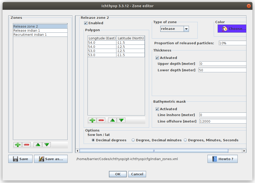
Zones can be added, edited or removed directly within the user interface (Figure 2.1).
2.1.3.1 Adding, removing and renaming zones
The number of zones is managed on the left part of the panel.
New zones can be added by clicking the  button. When a zone is selected, it can be removed by clicking on the
  button.
The reordering of the zones is achieved by clicking on the  and
and  buttons.
When double-clicking on the name of the zone on the left panel, the user rename a zone.
2.1.3.2 Editing a zone
When a zone is selected, the user can edit different parameters associated with the zone.
First, the user can enable or disable a zone by clicking on the Enabled tick box.
The zones are defined by providing the geographic points coordinates. Points can be added, removed and reordered by using the , , and buttons, respectively. The user can also change the format of the points coordinates by clicking on the radio buttons in the Options bottom panel.
Ichthyop uses three types of zones: one for release (see Section 5.2), one for recruitment of particles and one for orientation (see Section 6.3.1). This type is chosen by using the Type of zone combo box. For release zones, the user can specify the number of particles that will be released in the zone (only if the user_defined_nparticles parameter is set equal to true, cf Section 5.2). This is done by filling the Proportion of released particles textbox and pressing ENTER
Each zone is associated with a color for the preview and the display of the simulation results. This color can be edited by using the  button.
In the case of 3D simulations, the user can specify a subset of zone area based on a lower and upper depth. This feature is activated by clicking on the Activated tick box of the Thickness panel. The user can also specify a subset of zone area based on bathymetry (for example 0 to 200m, for using only the subset of zone area from 0 to 200 m depth). This feature is activated by clicking on the Activated tick box of the Bathymetric mask panel.
2.2 Running
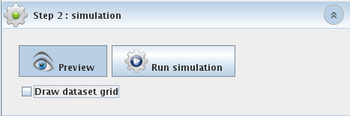
The user may first want to preview the simulated area by clicking on the “Preview” button. This is also a way to check that the simulation is correctly set up, i.e. that the application found all the parameters required for starting the simulation. More specifically, Ichthyop will attempt to read the geographical variables (longitude, latitude and depth) from the hydrodynamic dataset in order to draw the area. It should also display the release and the recruitment zones if they have been defined and activated in the configuration file. Make sure that what you see is what you expect, and go back to “Step 1: configure” if not.
When the preview is satisfactory, click on “Run simulation” for starting the simulation. The progress bar will give an estimation of the remaining time for the simulation to complete. You can interrupt (but not pause) the simulation anytime by a click on “Stop simulation”.
Depending on the capabilities of your computer, the number of released particles, how many actions are enabled, etc. the simulation may require a large amount of the available dynamic memory and the application may look like it is frozen. Wait until the simulation runs to completion. Refer to Section 4.1 if the application crashes because of memory issue.
2.3 Visualize results
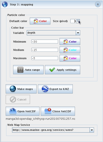
When the simulation is completed, the application automatically opens the current Ichthyop output file for visualizing the results. If your computer is connected to Internet, you should see the map being centered above the simulated area. Otherwise, it only displays a Grey background.
Click on “Open NetCDF” and select the Ichthyop output file you wish to visualize. When the NetCDF file is opened, the application brings you back to the exact point where it was when the simulation just completed.
The application offers two ways for visualizing the results :
Make maps, i.e. draw the successive locations of the particles on a map over time- Export the particle trajectories in a KMZ file that can be opened with Google Earth.
2.3.1 Results
Ichthyop archives the simulation outputs in NetCDF format, a machine-independent data formats for sharing array-oriented scientific data.
The NetCDF file is recorded in the Ichthyop output folder (set in the Output section of the configuration file) and the file name contains the date and time of the file creation.
Default content of the NetCDF output file is the time and, for each particle, the longitude and latitude, the mortality status and in case of 3D simulations, the depth
2.3.2 Particle color
The Default color button allows to set the particle color for visualizing the trajectories.
Particles are plotted as small circles. Particle size determines the diameter of the circle in pixel.
To use a colorbar, select in the Combo box a variable archived in the Ichthyop output file (e.g. depth or time) you wish to visualize as a tri-color range. The Auto range button will scan the values of this variable and suggest the following range : [mean - 2 * standard deviation; mean + 2 * standard deviation]. Do not forget to click on Apply settings for validating the changes of the color bar.
For taking off the color bar, select the None item in the Combo box and click on Apply settings. A click on Default color button also deactivates the color bar.
2.3.3 Make maps using Web Map Service
A Web Map Service (WMS) is a standard protocol for serving georeferenced map images over the Internet.
Ichthyop provides two different WMS for displaying the ocean bathymetry and the cost line as a background of the particle trajectories.
Maps can be intuitively zoomed in and out with the mouse wheel and re-centered doing a mere drag and drop.
Depending on the quality of the Internet connection and how busy is the Web Map Server, the display of the background tiles may take a while or even not work at all. In that case, try again with another WMS and change the zoom scale.
When the settings of the map look satisfactory, click on the Make maps button. Ichthyop will then create a folder that has exactly the same name as the simulation NetCDF output file (without the .nc extension) in the output directory and save the maps in this folder as PNG images.
Again, depending on the computer capabilities and the number of particles, the map creation may require a large amount of the available dynamic memory and the application may seem frozen. Wait for the application to complete this step. Refer to Section 4.1 if the application crashes because of memory issue.
2.3.4 Export trajectories to KMZ format
Click on Export to KMZ button for recording the particle trajectories into a KMZ file. The file is recorded in the same directory as the Ichthyop output file, with the same name and the .kmz extension. KMZ format is the standard file format for visualizing georeferenced information with GoogleEarth.
Color settings (default color or color bar) and particle size will also be stored in the KMZ file.
When the export is completed, browse to the output folder and click on the KMZ file for launching GoogleEarth (assuming the program is already installed on your computer).
2.4 Animation
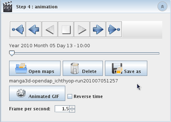
Click on “Open maps” and select the simulation output folder that contains the PNG pictures you wish to visualize. When the folder is opened, the application brings you back to the exact point where it was when the map creation just completed.
Set the number of frames per second of the animation with the spinner.
You can also create an animated GIF. The file is recorded in the same directory as the Ichthyop output file, with the same name and the “.gif” extension.