13 Interpolation of coordinates
There are two coordinate systems in Ichthyop:
- the grid coordinate, with
xranging from 0 tonx - 1andyranging from0tony - 1 - the geographical coordinates, i.e. longitude and latitude
In Ichthyop, there are fonctions that allows to switch from one system to another, considering that the grid may be irregular (for example NEMO or CROCO grid).
13.1 Grid to geographical coordinates
Conversion from grid to geographical coordinates is done by using the xy2latlon methods associated with Dataset objects.
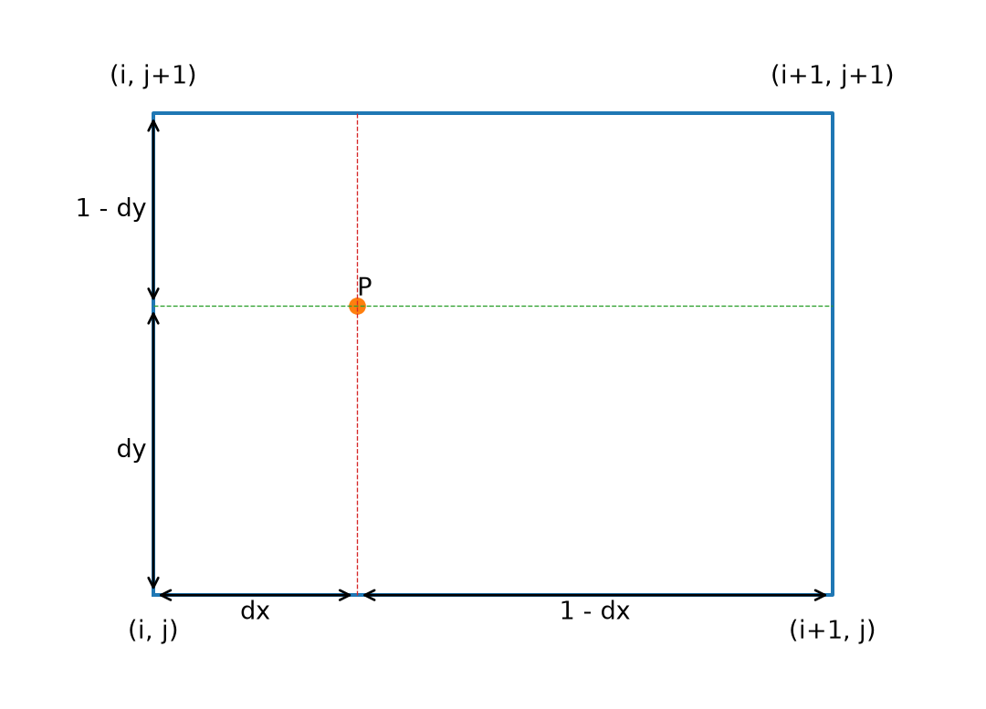
This function is a bilinear interpolation of the grid coordinates, as shown in Figure 13.1
The coordinate of the particle P is determined as a weighted mean of the coordinates of the four corners, with the weight being provided by the distance of the particle from the corners (dx dy). The closest the particle is to a corner, the more weight is has.
For example, the longitude of the particle \(lambda_P\) is given by:
\[ \lambda_P = (1 - dx)(1-dy) \lambda_(i, j) + dx(1-dy) \lambda_(i + 1, j) + (1 - dx)dy \lambda_(i, j+1) + dxdy \lambda_(i+1, j+1) \]
Note that by construction, the sum of the weight equals to 1, so no need to divide by the total weight.
13.2 Geographical to grid coordinates
The switch from geographical to grid coordinates is a bit more tricky, considering that the grid may be irregular. Let’s consider the example in Figure 13.2
The first step is to determine the coordinates of the cell in wich the particle is located. In the code, this is done by a dichotomic search. We first look in which quarter of the domain the particle is located. This quarter is then decomposed into 4 quarters, and we determine in which subquarter the particle is locate. At the end, the cell in which the particle is located is selected (Figure 13.2).
0.4285714285714282 0.42857142857142855
0.6428571428571432 0.6428571428571429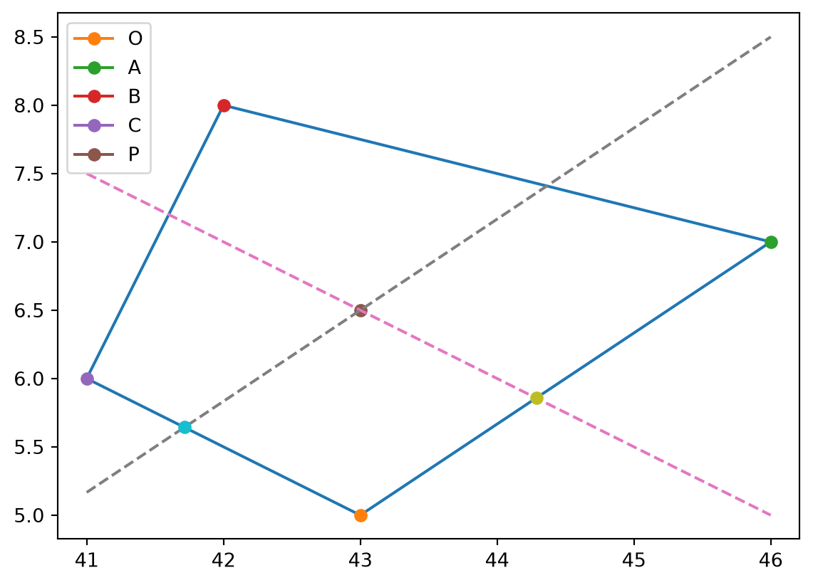
Each corner of the cell is given by a longitude and latitude \(\lambda_{i,j}, \phi_{i,j}\), while the particle has longitude and latitude given by \(\lambda_{P}, \phi_{P}\). The objective is to determine, given the geographical coordinates of the coordinates and of the particle, the \(\Delta x\) and \(\Delta y\) values of the particle, so that:
\[ x_P = i + \Delta x \]
\[ y_P = j + \Delta y \]
with \((x_P, y_P)\) the particle grid coordinate and \((i,j)\) the coordinate of the lower left corner.
We assume that:
\[ \mathbf{OP} = A \times \mathbf{OA} + B \times \mathbf{OC} \]
When using the geographical coordinates:
\[ \lambda_P - \lambda_O = \Delta X \times (\lambda_A - \lambda_O) + \Delta y \times (\lambda_C - \lambda_O) \tag{13.1}\]
and
\[ \phi_P - \phi_O = \Delta X \times (\phi_A - \phi_O) + \Delta y \times (\phi_C - \phi_O) \tag{13.2}\]
This is a system of 2 equations with two unknown (\(\Delta X\) and \(\Delta y\)). It is not resolved directly. Instead, we will look for the value of the longitude of the intersect of the straight line that crosses P and which is perpendicular to \(\mathbf{OC}\) with the straight line \(\mathbf{OA}\).
Based on the fact that each point \((X, Y)\) belonging to a straight line width a slope \((S_y, S_x)\), we have:
\[ X \times S_y - Y \times S_x = c \]
with \(c\) a constant, we can characterise these two straight lines with the known coordinates:
\[ \phi_P (\lambda_C - \lambda_O) - \lambda_P (\phi_C - \phi_O) = c1 \]
which characterize the line that crosses P and that is parallel to OC
\[ \phi_O (\lambda_A - \lambda_O) - \lambda_O (\phi_A - \phi_O) = c2 \]
which characterize the OA line.
Since the unknown point also is on these two lines, we can write
\[ \phi_I (\lambda_C - \lambda_O) - \lambda_I (\phi_C - \phi_O) = c1 \]
\[ \phi_I (\lambda_A - \lambda_O) - \lambda_I (\phi_A - \phi_O) = c2 \]
This is an equation with two unknown (\(\phi_I\) and \(\lambda_I\)) that can be solved using the Cramer formula. In this case, we are only interested in \(\lambda I\):
\[ \lambda_I = \frac{ c_2(\lambda_C-\lambda_O)-c_1(\lambda_A-\lambda_O) }{ (\lambda_A-\lambda_O)(\phi_C-\phi_O) -(\lambda_C-\lambda_O)(\phi_A-\phi_O) } \]
Finally, the grid increment is given as follows:
\[ \Delta x = \frac{(\lambda_I - \lambda_O)}{(\lambda_I - \lambda_A)} \]
The same operation is done to determine the latitude of \(\phi_J\) and hence the \(\Delta y\) grid increment.
Caution
Since the grid is irregular, the cell edges may not be orthogonal. Therefore, a simple projection does not work
Note
The equation could be resolved more easily using Equation 13.1 and Equation 13.2, also using Cramer’s formula:
\[ D = (lonA - lonO)(latC - latO) - (latA - latO)(lonC-lonO) \]
\[ D_x = (lonP - lonO)(latC - latO) - (lonC - lonO) (latP - latO) \]
\[ D_y = (lonA - lonO)(latP - latO) - (latA - latO) (lonP - lonO) \]
\[ \Delta x = \dfrac{D_x}{D} \]
\[ \Delta y = \dfrac{D_x}{D} \]