10 Grid management

10.1 Regular grid

10.2 NEMO grid

In this section, the main features of the NEMO grid and the implications in Ichthyop are summarized.

10.2.1 Horizontal

Computation domain

In the NEMO grid, the computation domain extends from the western edge of the western T cell (i=0) to the eastern edge of the eastern T cells (i=nx), and from the southern edge of the southern T cells (j=0) to the northern edge of the nothern T cells (j=ny).

Indexing

The horizontal layout of the NEMO grid is as follows:

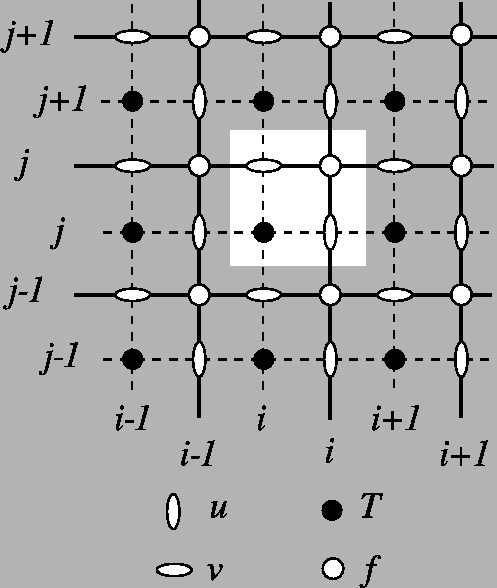
Tracer points (T points) are stored at the center of the cell. Zonal velocities (U points) are stored on the eastern face, while meridional velocities (V points) are stored on the northern face. U, V and T points have the same number of elements!

Scale factors

In NEMO, the zonal and meridional length of the cells are stored in the e1x and e2x variables, with x equals to t, u or v depending on the point considered.

Land-sea mask

For a particle at a given location, we determine whether it is on land as follows:

We extract the i index of the T land-sea mask to use by computing round(x - 0.5).
We extract the j index of the T land-sea mask to use by computing round(y - 0.5).
We extract the mask value at the (i, j) location.

Close to coast

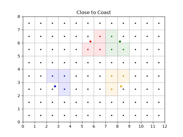
To determine whether a particle is close to coast, we extract the three neighbouring T cells. If one of them is land, then it assumed to be close to coast.

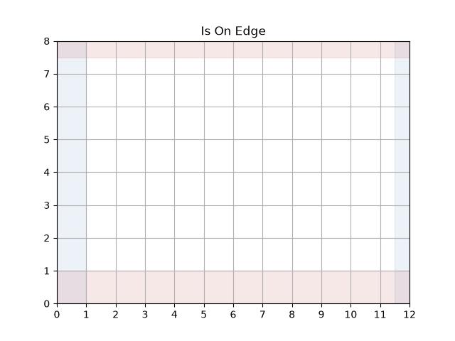
Is On Edge

The particle is considered to be out of the domain if the y value is greater than ny - 0.5 (no possible interpolation of T points) or less than 1 (no possible interpolation of V points).

If there is no zonal cyclicity, the particle is also considered to be out of the domain if the x value is greater than nx - 0.5 (no possible interpolation of T points) or less than 1 (no possible interpolation of U points).

Zonal cyclicity

For regional simulations, there is no zonal cyclicty. On the other hand, for global NEMO simulations, which runs on the ORCA grid, the zonal cyclicity is as follows (indexes are provided for T points):

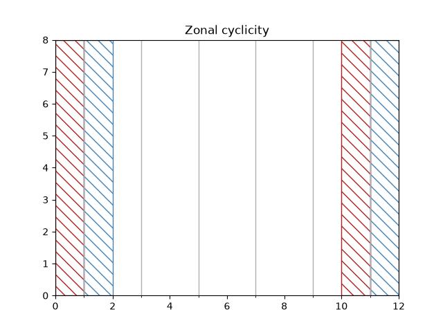
Therefore:

if \(x \leq 1\), the particle is moved at \(N_x - 2 + x\)
if \(x \geq nx - 1\), the particle is moved at \(x - N_x + 2)\)

Interpolation

Interpolation of T variables

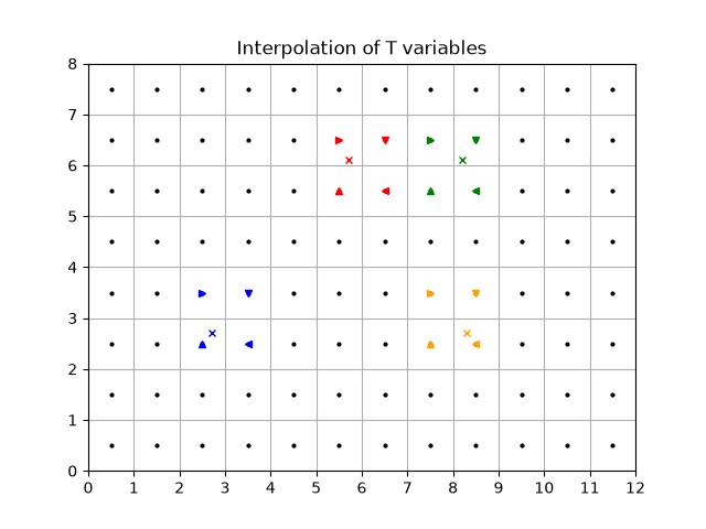
Given a given position index of a particle with the T grid, the determination of the interpolation is done as follows:

First, the i index of the T grid column left of the particle is found. This is done by using floor on the x - 0.5 value. The removing of 0.5 is to convert the x value from the computational grid to the T grid.
Then, the j index of the T grid line below the particle is found. This is done by using floor on the y - 0.5 value. The removing of 0.5 is to convert the y value from the computational grid to the T grid.
The area to consider is defined by the [i, i + 1] and [j, j + 1] squares.

An illustration is given below

Interpolation of U variables

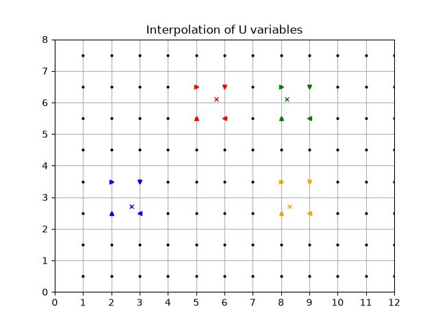
Interpolation of U variables is done as follows:

First, the i index of the U point left of the particle is found by using floor(x - 1). The -1 is to move from the computation grid to the U grid system.
Then, the j index of the U grid line below the particle is found. This is done by using floor on the y - 0.5 value. The -0.5 is to move from the computation grid to the U grid system.
The box used to average the variable is therefore defined by the [i, i + 1] and [j, j + 1] squares.

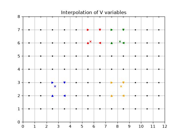
Interpolation of V variables

Interpolation of V variables is done as follows:

First, the i index of the V point left of the particle is found by using floor(x - 0.5). The -0.5 is to move from the computation grid to the U grid system.
Then, the j index of the V grid line below the particle is found. This is done by using floor on the y - 1 value. The -1 is to move from the computation grid to the U grid system.
The box used to average the variable is therefore defined by the [i, i + 1] and [j, j + 1] squares.

10.2.2 Vertical

Indexing

The original NEMO vertical indexing system is shown below:

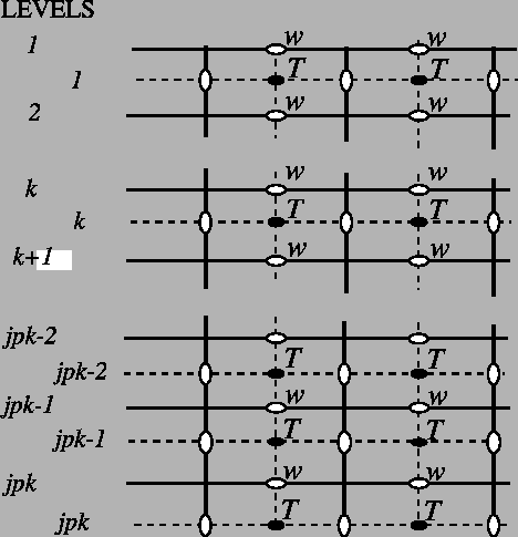
Index starts at 0 (at the surface) and ends at \(N_z - 1\) at depth. There are as many W levels as T levels. In NEMO, the T point situated at \(N_z - 1\) is always masked. W levels are located above the corresponding T points.

Therefore, in Ichthyop, only the first \(N_z - 1\) T points are read, while all the \(N_z\) W points are read. This is show below:

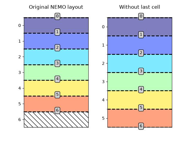
Vertical indexing system as used in Ichthyop. Red dashed lines represent the W levels (cell edges), whose index is given in the gray box.

There is now \(N_z\) W levels but \(N_z - 1\) T levels.

Furthermore, since in Ichthyop the first index corresponds to the seabed, the arrays are vertically flipped. Consequently, the final structure of the vertical grid is as follows:

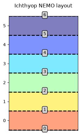
Corrected vertical indexing, with k=0 associated with the bottom depth.

Land-sea mask

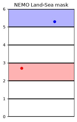
Vertical land-sea mask

Interpolation

T variables

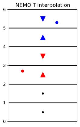
Vertical interpolation of T variables.

W variables

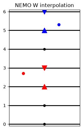:align: center :width: 250 px

Vertical interpolation of T variables.

10.3 ROMS grid

In this section, the main features of the ROMS grid and the implications in Ichthyop are summarized.

10.3.1 Horizontal

The horizontal grid layout, as described on the ROMS documentation, is shown in Figure 10.1:

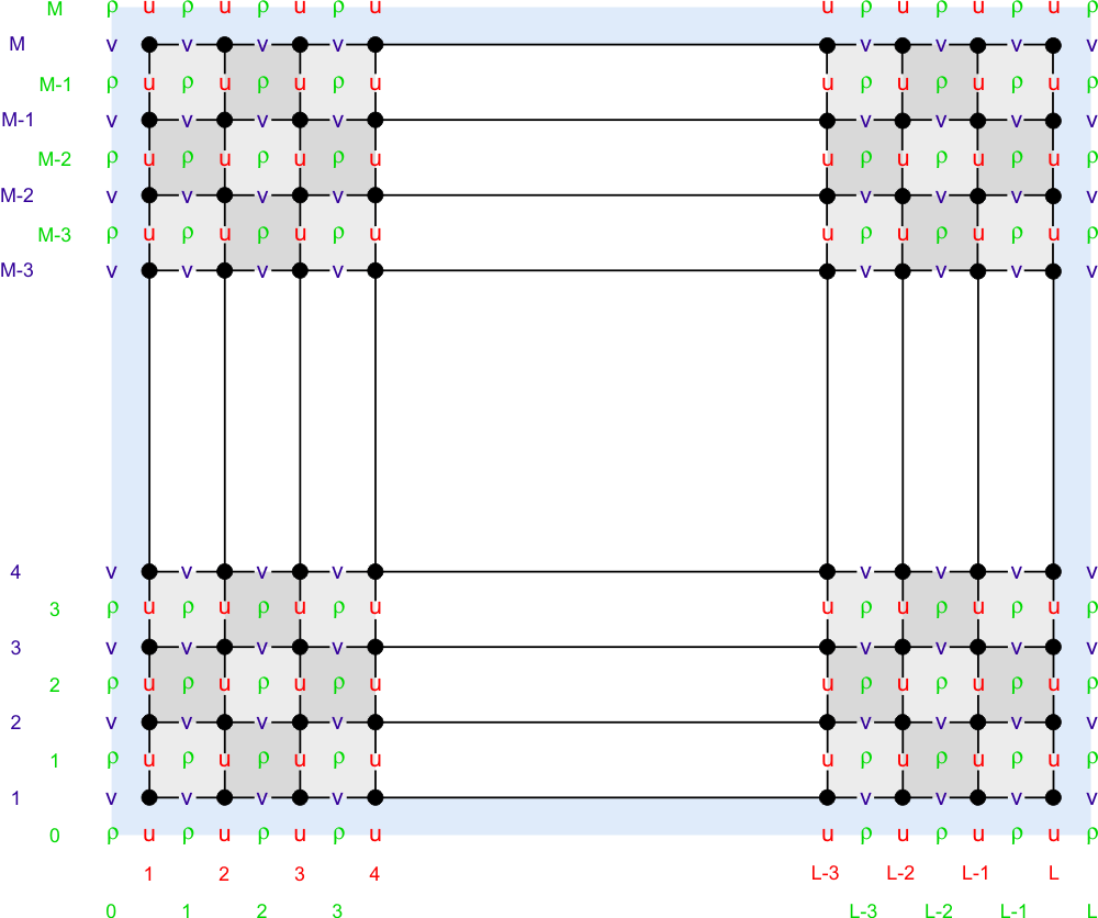
Figure 10.1: ROMS staggered grid structure

In Figure 10.2, the structure of the grid, based on Figure 10.1, is drawn with the indexes of the different points added.

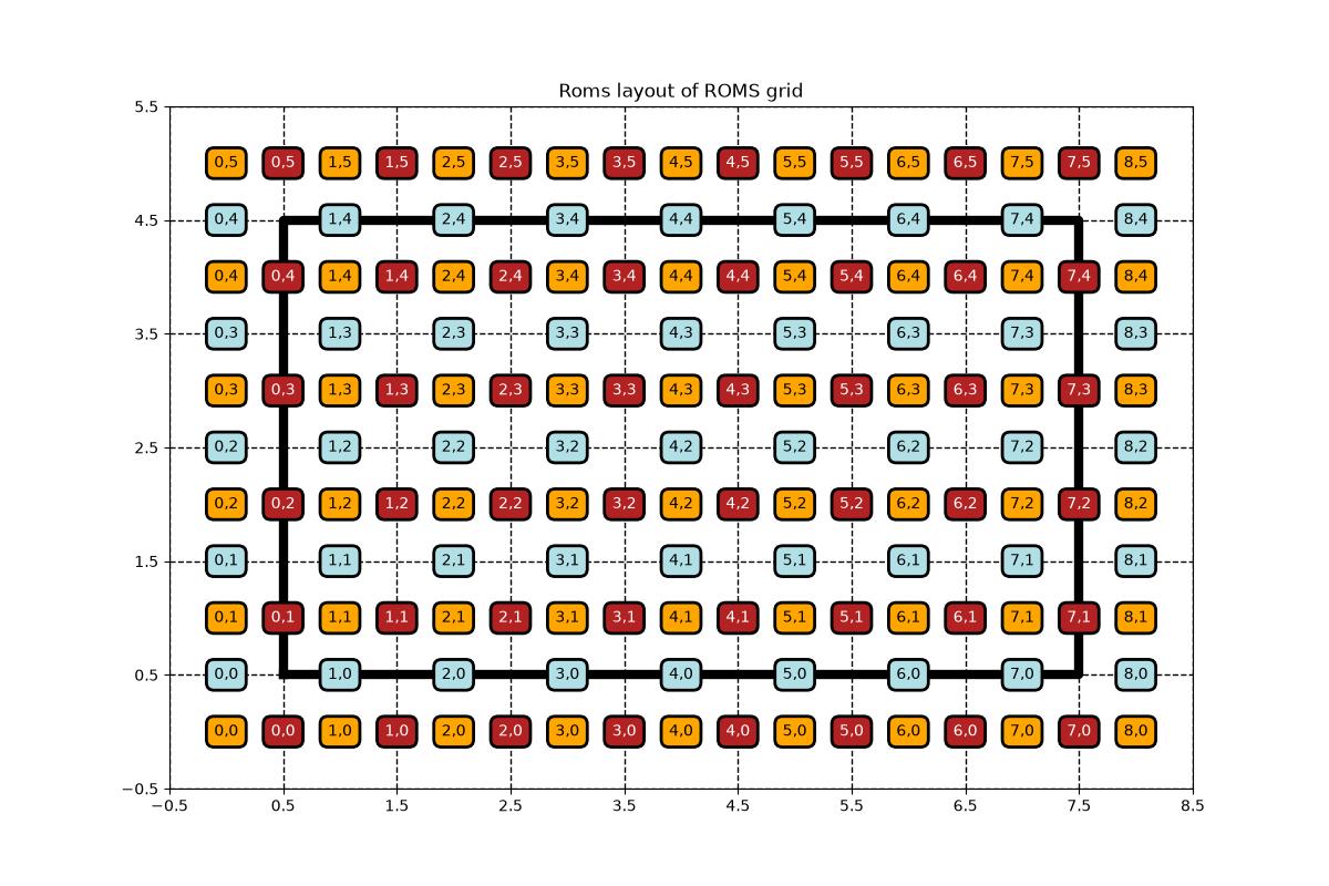
Figure 10.2: ROMS grid layout. T points are shown in orange, U points are shown in red and V points are shown in blue. The Ichthyop computation area is shown in black

In ROMS, there are 1 extra column of T points compared to U points. There also is 1 extra line of T points compared to V points.

10.3.1.1 Is on edge

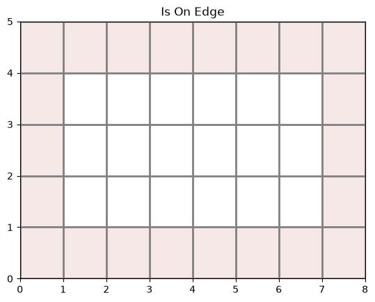
In Ichthyop, a particle is considered out of domain when U, V, or T points cannot be interpolated using a 4 point interpolation. Looking at the layout described in Figure 10.2, this occurs when:

\(x < 0.5\) or \(x > N_x -1 - 0.5\), when \(U\) values cannot be interpolated.
\(y < 0.5\) or \(y > N_y -1 - 0.5\), when \(V\) values cannot be interpolated.

The excluded domain is represented in Figure 10.3:

Figure 10.3: Excluded domain in the Ichthyop ROMS simulations.

10.3.1.2 Land-sea mask

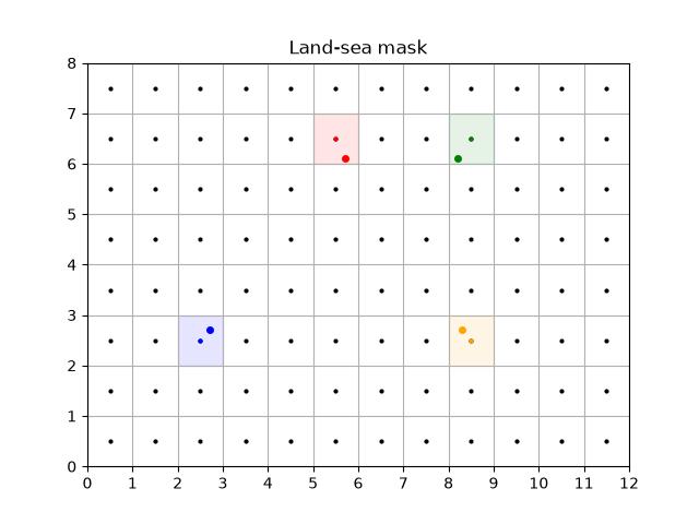
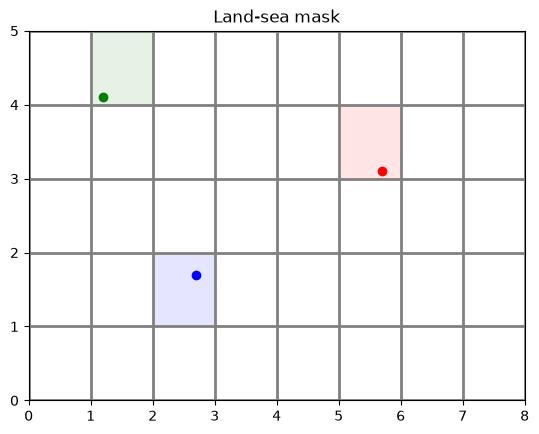
The land-sea mask of a particle is obtained by rounding the \(x\) and \(y\) position of the particle, and getting the value of the mask at these rounded indexes. Some examples are shown in Figure 10.4

Figure 10.4: Land-sea masking for ROMS grid

10.3.1.3 Interpolation

In this section, we describe how the zonal and meridional velocity fields are interpolated.

T interpolation

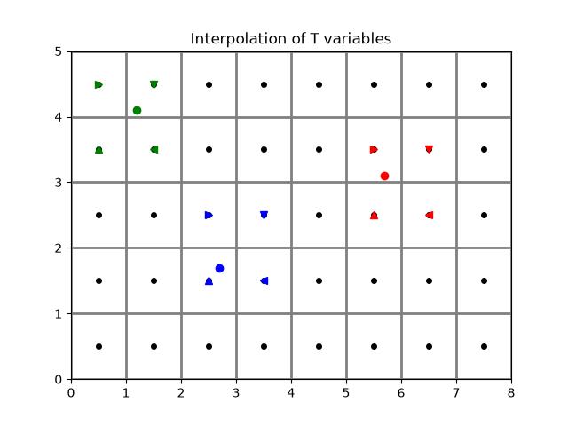
Given a given position index of a particle with the T grid, the determination of the interpolation is done as follows:

First, the i index of the T grid column left of the particle is found. This is done by using floor on the x value.
Then, the j index of the T grid line below the particle is found. This is done by using floor on the y value.
The area to consider is defined by the [i, i + 1] and [j, j + 1] squares.
The weights are given by considering the coordinate distance between the particle location and the targeted T points.

An illustration is given Figure 10.5.

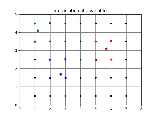
Figure 10.5: Interpolation of T points from ROMS grid

U interpolation

Interpolation of U variables is done as follows:

First, the i index of the U point left of the particle is found. This is done by using floor(x - 0.5). The -0.5 is to move from the computation T grid to the U grid system (if \(x=0.5\) in T system, \(x=0\) in U system).
Then, the j index of the U grid line below the particle is found. This is done by using floor on the y value.
The box used to average the variable is therefore defined by the [i, i + 1] and [j, j + 1] squares.

An illustration is given Figure 10.6.

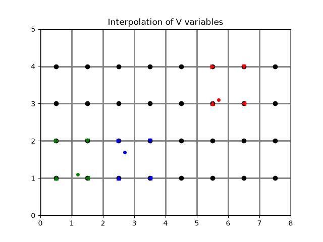
Figure 10.6: Interpolation of U points from ROMS grid

V interpolation

Interpolation of V variables is done as follows:

First, the i index of the V point left of the particle is found by using floor(x).
Then, the j index of the V grid line below the particle is found. This is done by using floor on the y - 0.5 value. The -0.5 is to move from the computation T grid to the V grid system (if \(y=0.5\) in T system, \(y=0\) in V system).
The box used to average the variable is therefore defined by the [i, i + 1] and [j, j + 1] squares.

An illustration is given Figure 10.7.

Figure 10.7: Interpolation of V points from ROMS grid

10.3.2 Vertical

10.3.2.1 Sigma coordinate

The vertical coordinate system of ROMS is discussed on WikiRoms and shown below.

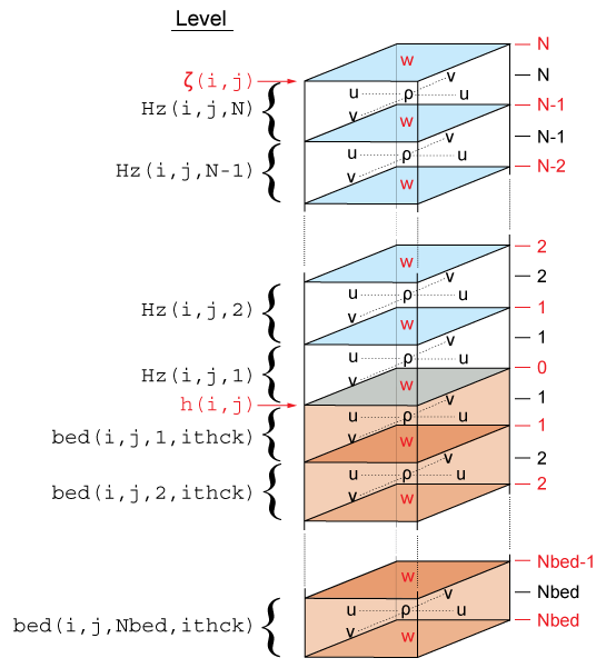
The vertical coordinate in ROMS is \(\sigma\), which varies between \(-1\) (ocean bottom) and \(0\) (ocean surface). There are two implementations of the \(\sigma\) to \(z\) conversion, both using sea-level anomalies (\(\zeta\)) and bathymetry (\(h\)).

The first one is available in ROMS since 1999 and is given by:

\[ z(x,y,\sigma,t) = S(x,y,\sigma) + \zeta(x,y,t) \left[1 + \dfrac{S(x,y,\sigma)}{h(x,y)}\right] \]

with

\[ S(x,y,\sigma) = h_c \, \sigma + \left[h(x,y) - h_c\right] \, C(\sigma) \]

and \(h_c\) and \(C(\sigma)\) parameters provided in the grid file.

The second transform, called UCLA-ROMS, is given by:

\[ z(x,y,\sigma,t) = \zeta(x,y,t) + \left[\zeta(x,y,t) + h(x,y)\right] \, S(x,y,\sigma) \]

with

\[ S(x,y,\sigma) = \dfrac{h_c \, \sigma + h(x,y)\, C(\sigma)}{h_c + h(x,y)} \]

and \(h_c\) and \(C(\sigma)\) parameters provided in the grid file.

It can be rewritten in the same form as the original one.

\[ z(x,y,\sigma,t) = h(x,y) S(x,y,\sigma) + \zeta(x,y,t) + \zeta(x,y,t) S(x,y,\sigma) \]

\[ z(x,y,\sigma,t) = h(x,y) S(x,y,\sigma) + \zeta(x,y,t) \left[1 + S(x,y,\sigma)\right] \]

\[ z(x,y,\sigma,t) = h(x,y) S(x,y,\sigma) + \zeta(x,y,t) \left[1 + \dfrac{h(x, y)S(x,y,\sigma)}{h(x, y)}\right] \]

In this form, both formulations can be expressed as:

\[ z(x,y,\sigma,t) = H_0(x, y, \sigma) + \zeta(x,y,t) \left[1 + \dfrac{H_0(x, y, \sigma)}{h(x, y)}\right] \]

with \(H_0\) which is constant overt time, and which varies between the classical and the UCLA formulations. For the classical formulation:

\[ H_0(x, y, \sigma) = S(x, y, \sigma) \]

For the UCLA formulation:

\[ H_0(x, y, \sigma) = h(x, y) S(x, y, \sigma) \]

10.3.2.2 Interpolation

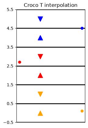
In Ichthyop, the vertical index ranges from 0 (center of the bottom T cell) to \(N_z - 1\) (center of the surface T cell).

Interpolation of T variables on the vertical is done as follows:

First, the index of the T cell just below is obtained by using the floor function on the Z index.
Then, the value is interpolated between the cell below and above.

An example is shown in Figure 10.8

Figure 10.8: Vertical interpolation of T points on ROMS grid

10.3.3 Vertical velocity reconstruction

Vertical velocity, if not provided by the user, can be reconstructed from zonal and meridional velocities.

The continuity equation in terrain following coordinated gives (cf Roms doc):

\[ \dfrac{\partial}{\partial \sigma} \left(\frac{H_z\ \Omega}{mn}\right) = -\dfrac{\partial}{\partial t} \left(\frac{H_z}{mn}\right) - \dfrac{\partial}{\partial \xi} \left(\frac{H_z\ u}{n}\right) - \dfrac{\partial}{\partial \eta} \left(\frac{H_z\ v}{m}\right) \tag{10.1}\]

with \(\Omega\) the vertical velocity in sigma coordinate, \(H_z = \dfrac{\partial z}{\partial \sigma}\) and \(m\) and \(n\) the ROMS/CROCO scale factors. Let’s define the vertical flux (in \(m^3.s^{-1}\)) as:

\[ F_z =\frac{H_z\ \Omega}{mn} \]

The vertical integration of Equation 10.1 gives:

\[ {F_z}\left(s=k\right) = F_z\left(s=0\right) - \int_{s=-1}^{s=k} \left[\dfrac{\partial F_z}{\partial t} + \dfrac{\partial}{\partial \xi} \left(\frac{H_z\ u}{n}\right) + \dfrac{\partial}{\partial \eta} \left(\frac{H_z\ v}{m}\right) \right] \tag{10.2}\]

assuming that \(F_z(s=-1) = 0\) (i.e. no flux of water at the surface).

In Ichthyop, the \(\dfrac{\partial F_z}{\partial t}\) term is not considered, since it cannot be computed considering that free-surface is not saved at a sufficient temporal resolution. Therefore, Equation 10.2 simplifies as follows:

\[ F_z(s=k) = F_z(s=0) - \int_{s=-1}^{s=k} \left[ \dfrac{\partial}{\partial \xi} \left(\frac{H_z\ u}{n}\right) + \dfrac{\partial}{\partial \eta} \left(\frac{H_z\ v}{m}\right) \right] \tag{10.3}\]

Due to the different approximations, the vertical flux at the sea-surface \(F_(N_Z)\) is not 0 at it should be. This is what is called in the ROMS/CROCO community the “grid breathing”. Since the sigma levels vary as a function of sea-surface height, we need to substract this “breathing” component from out vertical flux calculation.

This residual flux is therefore removed at each depth index, linearly as a function of depth. The correction applied is given by:

\[ C(s=k) = ({Z_w(k) - Z_w(0)})\dfrac {F_z(s=N_Z)} {Z_w(N_Z) - Z_w(0)} \]

with

\[ \dfrac {F_z(s=N_Z)} {Z_w(N_Z) - Z_w(0)} \]

the residual volume flux per unit depth. Therefore, the corrected vertical flux is:

\[ F_{z_{cor}} = F_z - C(s=k) \]

With this correction, we insure that the vertical flux is 0 at the surface. The physical interpretation of this correction is that when integrating the horizontal divergence equation, contributions due to the “grid breathing” will accumulate. Which is why the correction is proportional to the distance from the bottom.

The vertical velocity in \(\sigma\) coordinates \(Omega\) is computed as follows:

\[ \Omega(s=k) = \dfrac{F_{{z_{cor}}}(s=k) \times m \times n}{H_z} \]

The vertical velocity in \(z\) is given by:

\[ w = \dfrac{\partial z}{\partial t} + u \dfrac{\partial z}{\partial x} + v \dfrac{\partial z}{\partial y} + H_z \Omega \]

We neglect the isopycnal slope corrections and free surface tendency, and approximate:

\[ w = H_z \Omega \]

Finally, the vertical velocity is therefore given by:

\[ w(k) = F_{{z_{cor}}}(s=k) \times m \times n \]

10.4 MARS grid

In this section, the main features of the MARS grid and the implications in Ichthyop are summarized.

10.4.1 Horizontal

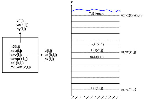
In MARS, the 3D structure of the grid is the same as the one in NEMO:

10.4.2 Vertical

The vertical coordinate of the Mars model is called \(\sigma\), which varies from -1 at seabed to 0 at the surface. In MARS, if the number of T points on the vertical is kmax, the number of W points is kmax + 1. For a given T cell located at the k index, the corresponding W point is located below. k=0 corresponds to the bottom, while k=kmax corresponds to the surface.

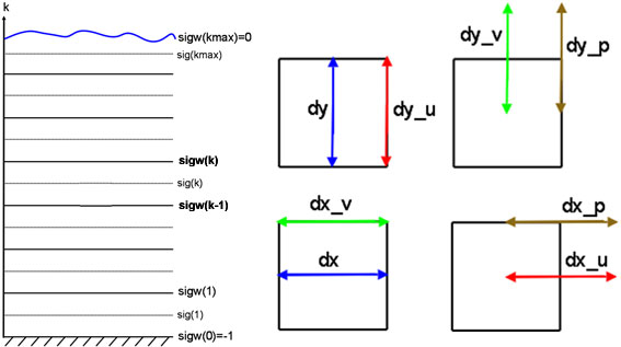
The conversion from \(\sigma\) to \(z\), using generalized \(\sigma\) levels, is given in Dumas (2009) (equation 1.29):

\[ z = \xi (1 + \sigma) + H_c \times [\sigma - C(\sigma)] + H C(\sigma) \]

where \(\xi\) is the free surface, \(H\) is the bottom depth and \(H_c\) is either the minimum depth or a shallow water depth above which we wish to have more resolution. \(C\) is defined as (equation 1.30):

\[ C(\sigma) = (1 - \beta) \dfrac{\sinh(\theta \sigma)}{\sinh(\theta)} + \beta \dfrac{\tanh[\theta(\sigma + \frac{1}{2})]-\tanh(\frac{\theta}{2})}{2 \tanh(\frac{\theta}{2})} \]

However, if the \(H_c\) variable is not found, the following formulation will be used:

\[ z = \xi (1 + \sigma) + \sigma H \]

Note that the \(C(\sigma)\) variable is read from the input file.

10.5 FVCOM grid

In the Ichthyop repository (https://github.com/ichthyop/ichthyop), there is a feature branch, called feature/fvcom-grid, which allows to use the unstructured mesh grid from the FVCOM model.

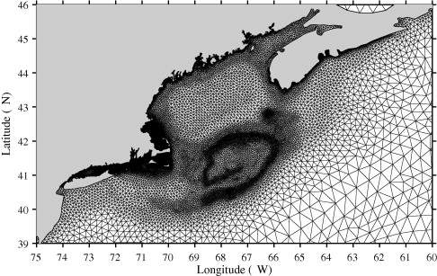
Figure 10.9: Example of unstructered FVCOM grid. Source: Qi et al. (2009)

In order to use Ichthyop with FVCOM grid, you will need to download this specific branch and compile the code manually (see Section 1.2.2).

In the present section, we describe some features of how tracer and velocity fields are computed. The authors acknowledge Laki Premathilake for his very important contribution and his very kind help.

10.5.1 Scale factors description

The FVCOM grid is associated with shape functions that are used to interpolate vector (i.e. velocities) and scalar properties (i.e. temperature) at given locations. These scale factors are

\(a1u(N, 4)\), \(a2u(N, 4)\), \(aw0(N_e, 3)\), \(awx(N_e, 3)\) and \(awy(N_e, 3)\) with \(N\) the number of elements (i.e. triangles) defined in the grid and \(N_{e}\) the number of nodes.

10.5.2 Velocity computations

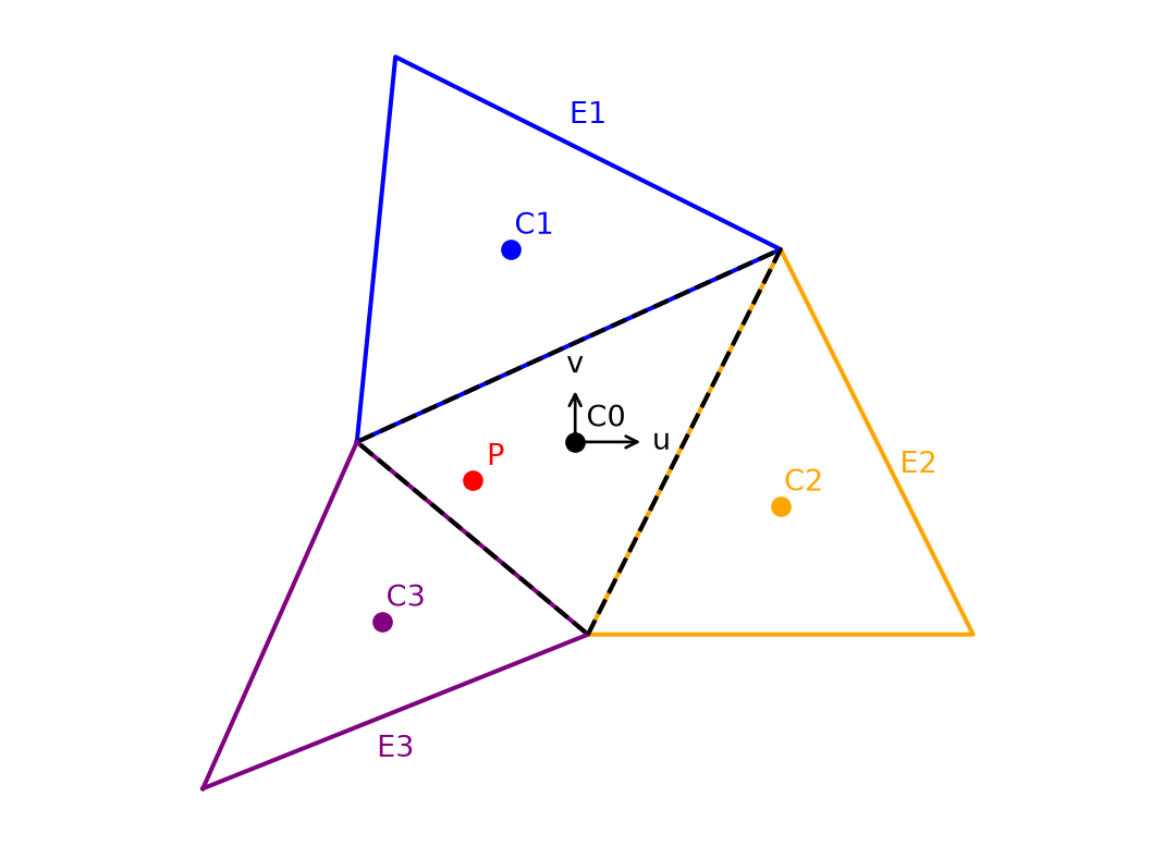
To compute the velocity field at the particle location, we first determine in which triangle the particle belongs (black triangle in Figure 10.10) and we also determine the neighbouring triangles (E1, E2 and E3 in Figure 10.10).

We compute the relative distance of the particle relative to the centroid of the triangle to which it belongs:

\[ \overline{X} = X_P - X_O \]

\[ \overline{Y} = Y_P - Y_O \]

Then, using the scale factors and velocity fields of the 4 triangles, the derivative of the velocity fields are computed at a given depth \(L_i\)

\[ \dfrac{dU}{dX} = a1u(E_0, 0) \times U(E_0, L_i) + a1u(E_1, 1) \times U(E_1, L_i) + a1u(E_2, 2) \times U(E_2, L_i) + a1u(E_3, 3) \times U(E_3, L_i) \]

\[ \dfrac{dU}{dY} = a2u(E_0, 0) \times U(E_0, L_i) + a2u(E_1, 1) \times U(E_1, L_i) + a2u(E_2, 2) \times U(E_2, L_i) + a2u(E_3, 3) \times U(E_3, L_i) \]

\[ \dfrac{dV}{dX} = a1u(E_0, 0) \times V(E_0, L_i) + a1u(E_1, 1) \times V(E_1, L_i) + a1u(E_2, 2) \times V(E_2, L_i) + a1u(E_3, 3) \times V(E_3, L_i) \]

\[ \dfrac{dV}{dY} = a2u(E_0, 0) \times V(E_0, L_i) + a2u(E_1, 1) \times V(E_1, L_i) + a2u(E_2, 2) \times V(E_2, L_i) + a2u(E_3, 3) \times V(E_3, L_i) \]

Finally, the velocity at the particle location is given by:

\[ U_P = U(E_0, L_i) + \dfrac{dU}{dX}\overline{X} + \dfrac{dU}{dY}\overline{Y} \]

\[ V_P = V(E_0, L_i) + \dfrac{dV}{dX}\overline{X} + \dfrac{dV}{dY}\overline{Y} \]

The first neighbouring element E1 corresponds to the neighbour relative to the first edge of the inner triangle, E2 corresponds to the neighbour relative relative to the second edge, and so on. To be confirmed?

10.5.3 Tracer computation

Interpolation of tracer fields can be done by using \(aw0\), \(awx\) and \(awy\). In the model, tracer fields are computed at the nodes of the triangles.

First, we find the triangle to which the particle belongs (black triangle in Figure 10.11).

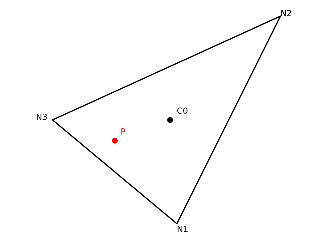
First, we compute the distance of the particle to the center of the triangle:

\[ \overline{X} = X_P - X_O \]

\[ \overline{Y} = Y_P - Y_O \]

Then, we compute the temperature at the center of the triangle as follows:

\[ T_O = aw0(E_0, 0) \times T(N_1, L_i) + aw0(E_0, 1) \times T(N_2, L_i)+ aw0(E_0, 2) \times T(N_3, L_i) \]

We also compute the tracer derivative as follows:

\[ \frac{dT}{dX} = awx(E_0, 0) \times T(N_1, L_i) + awx(E_0, 1) \times T(N_2, L_i) + awx(E_0, 2) \times T(N_3, L_i) \]

\[ \frac{dT}{dY} = awy(E_0, 0) \times T(N_1, L_i) + awy(E_0, 1) \times T(N_2, L_i) + awy(E_0, 2) \times T(N_3, L_i) \]

Finally, the tracer field at the particle location is given by:

\[ T_P = T_O + \frac{dT}{dX}\times \overline{X} + \frac{dT}{dY}\times \overline{Y} \]